DMAX in Google Sheets

What is DMAX in Google Sheets?

The DMAX function in Google Sheets works by returning the largest number from a specified column in a range that matches the given criteria. The function treats your data as a structured table where each column has a header, and each row is a record.

For example, if you have a list of products, their prices, and categories, you can use DMAX to find the highest price within a specific category. You just define the range, the column index to check, and the criteria range containing your filter conditions. This function is very useful for finding maximum values in scenarios like finding the highest sales figure of a salesperson and to get the maximum discount that is applied to any product in each category. Here, we find the product with the highest price, above a specified criterium, as shown below.

Syntax

The syntax of the DMAX function is as follows:

=DMAX(database, field, criteria)

The arguments include:

• database (mandatory) – The range of cells that makes up the database or list, including column headers (fields) and the data rows beneath them.
• field (mandatory) – The column to use for finding the maximum value. This can be given as the column header name in double quotes (e.g., “Price”) or as a column index number within the database range (e.g., 2).
• criteria (mandatory) – The range of cells containing the conditions to match. The criteria range must include at least one column label and the condition(s) beneath it.

How to Use DMAX Function in Google Sheets?

The DMAX function in Google Sheets returns the largest number from a given column that meets certain user-defined criteria. It is useful when you want to filter data based on conditions and then extract the highest value matching those conditions. You can use DMAX in two main ways:

• Enter DMAX manually
• Use the function from the Google Sheets menu

Enter DMAX Manually

To calculate the maximum value meeting specific criteria in Google Sheets manually, follow these steps:

Step 1: Enter the required details into the sheet, ensuring you have column headers.

Step 2: Click on the cell where you want the DMAX result to appear. Now, type =DMAX( into the cell.

=DMAX(

Step 3: Enter the arguments in the order specified in the syntax.

Here, we enter,

=DMAX(A1:D10, “Final Price”, F1:F2)

Here, A1:D10 is the database, “Final Price” is the column to search, and F1:F2 is the criteria range specifying the item name.

Step 4: Press Enter. It will return the highest value in the specified column that matches the criteria.

Entering DMAX Through the Menu Bar

1. Click on the cell where you want the result to appear.
2. Go to Insert > Function > Database > DMAX.
3. Fill in the arguments (database, field, criteria).
4. Press Enter, and your result will appear.

Examples

DMAX filters the database based on the conditions defined in the criteria range. Let us look at some practical examples to understand its uses.

Example #1

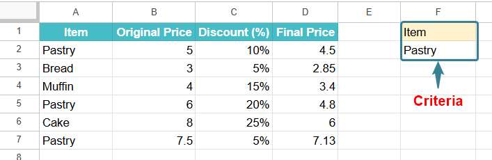
Let us look at an interesting example where we have the data from some items sold at a bakery. The bakery introduces a discount. We must find the highest final price of a specific product after applying discounts.

Step 1: Enter the details of the bakery in A1:D7. Then in F1:F2, create the criteria table with “Item” in F1 and “Pastry” in F2.

Step 2: Click on the cell where you want the result to appear and type the following formula:

=DMAX(A1:D7, “Final Price”, F1:F2)

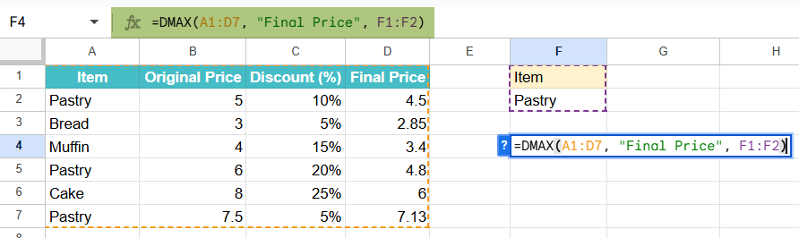
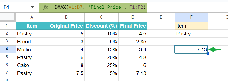
Step 3: Press Enter. The result will be 7.13, which is the highest final price among all entries for Pastry.

In short, DMAX in Google Sheets helps quickly find the highest final price for a bakery item that meets your chosen criteria, making it easy to spot top-priced products like the costliest pastry in seconds.

Example #2 – Using DMAX with Multiple Criteria

IN a sports equipment store that operates in multiple locations, we have details of the performance of the different stores in terms of sales. We must find the highest number of units sold based on two different conditions. Here the conditions we specify are as follows:

• Sales from the New York store for any product sold after 01/06/2024.
• Sales of basketballs from any of the stores after 15/07/2024.

We’ll use the DMAX function in Google Sheets to check both conditions and return the largest value found.

Step 1: Enter your sales details in Google Sheets as shown below:

Step 2: In another part of the sheet, we enter the criteria range as shown below.

Product/Store     Date of Sale

New York             >01/06/2024

Basketball           >01/06/2024

Step 3: Apply the DMAX formula as shown below:

=DMAX(A1:D9, “Units Sold”, F1:H3)

Where:

1. A1:D9: Range with data
2. “Units Sold” → The column from which we want the maximum value
3. F1:H3 → The criteria range

Step 4: Press Enter. The formula checks both sets of criteria and returns the value, which is the maximum number of units sold that meets either condition.

Explanation

Rows matching Condition 1 (New York sold after 01/06/2024) are given.

Rows matching Condition 2 (Basketballs after 01/06/2024) are highlighted in green.

DMAX considers both conditions and finds 215, which comes from a Chicago Basketball sale on 15/07/2024.

Example #3 – Using DMAX with Conditional Formatting

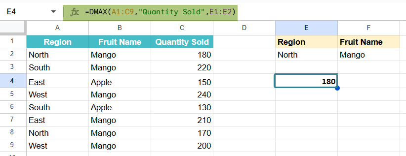
There is a fruit business, the details of which are mentioned in a sheet. We must highlight the row that contains the highest quantity sold for a given fruit type in a particular date range. Here, we want to see the largest sale of mangoes that happened in the North region. Let us use DMAX to calculate the highest value, and then conditional formatting to automatically highlight that row in the sheet.

Step 1: Enter the fruit sales data in Google Sheets as follows:

Step 2: Set the criteria range as in the other examples.

Fruit Name         Region

Mango                  North

This means we must find the largest mango sale in the North region.

Step 3: Type the following formula:

=DMAX(A1:C9, “Quantity Sold”, E1:F2)

1. A1:C9 represents the range.
2. “Quantity Sold” is the column we want the maximum value from
3. E1:F2 is the criteria range

Press Enter to get the result.

Step 4: Let us apply conditional formatting. Select the entire data table (A2:C9).

1. Go to Format → Conditional formatting.
2. Under Format cells if… choose Custom formula is.
3. Enter the formula: =$C2=$E$4
4. Choose a fill color to highlight the row with the highest sale and click done.
5. Now the row with the highest Mango sale after 01/07/2024 will be highlighted automatically.

By combining DMAX with conditional formatting, one can identify and visually highlight the top-performing sales records in Google Sheets.

Important Things to Note

1. The DMAX function can be used to extract the maximum value from large financial datasets, for example, to find the highest closing stock price for a specific company over a defined period.
2. ‍Unlike the DMAX function, the MAXIFS function does not need a structured database but works best with a simple range of cells.
3. The search criteria’s header name should match the database’s corresponding one.

Frequently Asked Questions (FAQs)

Download Template

This article must help understand DMAX Function in Google Sheets with its formulas and examples. You can download the template here to use it instantly.

Recommended Articles

Guide to What is DMAX Function in Google Sheets. We learn how to use DMAX function in google sheets with step-wise examples. You can learn more from the following articles. –

SUMPRODUCT in Google Sheets

NOMINAL in Google Sheets

FVSCHEDULE in Google Sheets