What Is Column Letter To Number In Excel?
Excel column to number involves converting column headers, denoted by one, two, and three letters, into numbers in ascending order, with column A being 1 and so on.
Users can change column letters to numbers in Excel to specify the required columns correctly in formulas and functions. Also, using the numeric values of the columns helps organize and manage massive data in a sheet better.
📥Download the ready-to-use Excel template to practice this tutorial yourself.
Excel-Column-To-Number
For example, the following table shows the sales figures at the branch offices of a firm from 2010-2022.

The dataset is large, with the branch office-wise total sales data at the end of the dataset.
The requirement is to give the users the numeric value of the column containing the branch office-wise total sales data so they can refer to it easily and quickly. Assume the target cell to display the required column number is cell B8.
Then, we can convert Excel column to number using the Excel COLUMN function in the target cell to obtain the required output.

In the above convert Excel column to number example, we know that the branch office-wise total sales data is in column O.
So, we apply the COLUMN() in cell B8, with the cell reference to a cell in column O supplied as the function argument.
It returns column O’s numeric value, 15, as the required outcome.
Table of contents
Key Takeaways
- The Excel column to numberconversion is the method to change the column letters to the corresponding numeric values.
- Users can convert column letters to numeric values to improve data organization and simplify data referencing in a worksheet.
- We can use the COLUMN() to achieve the required numeric value of a specific column. On the other hand, applying the function as an array formula gives the numbers of all the columns in the specified range.
- We can use the COLUMN function with other inbuilt functions such as INDIRECT, MATCH, INDEX, and ADDRESS to create formulas that return a column number.
How To Find Column Number In Excel?
The steps to find the Excel column to number are as follows:
- Choose a target cell to display the column number.
- Type =COLUMN( in the target cell. [ Alternatively, type =CO or =COL and double-click the COLUMN function from the listed Excel suggestions.]
- Enter the argument as a cell value or reference and close the bracket.
But when the requirement is to determine the current column number, we do not need to pass any argument value to the function. Instead, we can close the bracket. - Press Enter to view the required column number in the target cell.
Please note that a convert Excel column to number VBA macro will give us a custom function to determine the required output. However, using the COLUMN() is a more straightforward method. The former is useful for creating user-defined functions.
Examples
Check out the following Excel column to number examples to use the option effectively.
Example #1
Here are three scenarios of converting an Excel column to number using the COLUMN().
The following table contains the descriptions of the required column numbers.
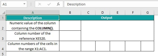
And we must show the results in the cells under the heading Output.
Then, the steps are as follows:
Step 1: Choose cell B2 and enter the COLUMN() without an argument value.
=COLUMN()

Next, press Enter to view the numeric value of the column containing the current cell, where we entered the COLUMN().

Step 2: Choose cell B3 and enter the COLUMN().
=COLUMN(XES20)
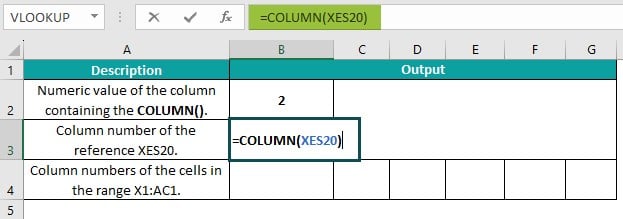
Press Enter to obtain the required output.

The function accepts the cell reference specified in the description in cell A3 and returns the corresponding numeric value of column XES, 16373.
Step 3: Choose the cell range B4:G4 and enter the COLUMN().
=COLUMN(X1:AC1)
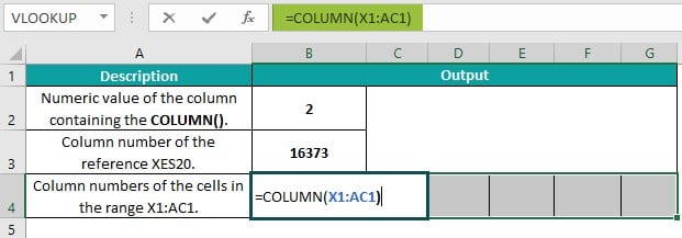
Next, execute the function as we would implement array formulas in Excel, i.e. by pressing Ctrl + Shift + Enter.
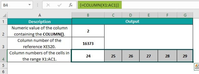
The function accepts the cell range reference specified in the description in cell A4. So, the array formula updates the corresponding numeric value of columns X:AC in the target cell range B4:G4.
Though a convert Excel column to number VBA code can help change a column name to a number, we can use the COLUMN() with other inbuilt functions to get the results quickly.
Example #2
The following table shows two sets of values and the arithmetic operations performed with the specified values in each row.

The requirement is to determine the column numbers of the arithmetic operations outcome and display the result in column E.
Then, the steps are as follows:
Step 1: Choose cell E2 and enter the following formula.
=”The column number of the cell containing the sum of the values 5000 and 2000 is “&COLUMN(INDIRECT(“D”&”2″))&”.”
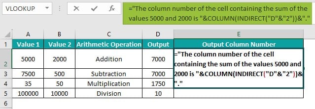
Press Enter to view the required column number.

Step 2: Choose cell E3 and enter the following formula.
=”The column number of the cell containing the difference between the values 7500 and 500 is “&COLUMN(INDIRECT(“D”&”3″))&”.”

Press Enter to view the required column number.

Step 3: Choose cell E4 and enter the following formula.
=”The column number of the cell containing the product of the values 35 and 50 is “&COLUMN(INDIRECT(“D”&”4″))&”.”

Press Enter to view the required column number.

Step 4: Choose cell E5 and enter the following formula.
=”The column number of the cell containing the division of the value 100000 by 10000 is “&COLUMN(INDIRECT(“D”&”5″))&”.”

Press Enter to view the required column number.
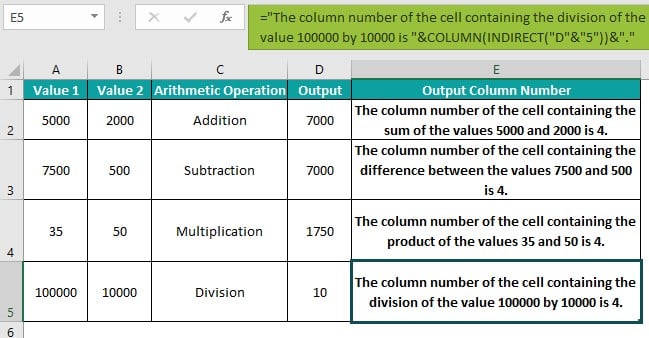
Let us check the cell E5 formula to understand how it works.
First, the INDIRECT function returns the Excel absolute reference of cell D5, $D$5. And then, the COLUMN() performs the Excel column to number conversion and returns the column number of cell reference $D$5, 4.
Finally, the text in the double quotations gets appended to the COLUMN() return value to give the output in cell E5.
Example #3
The following Excel column to number example involves a table listing column headers indicated by letters.

Then, here is how to convert the column letters to numbers and display them in column B.
Step 1: Choose cell B2 and enter the following MATCH excel function containing the INDEX excel function, ADDRESS Excel function, and COLUMN().
=MATCH(A2&”2″,ADDRESS(2,COLUMN($1:$1),4),0)

And using Ctrl + Shift + Enter, execute the expression as an array formula.

Step 2: Using the Excel fill handle, update the array formula in the remaining target cells B3:B7.

Let us check the cell B7 expression to understand how the formula works.
First, the column name in cell A7, VWO, gets concatenated with the number 2, resulting in the cell reference VWO2. And the COLUMN($1:$1) function returns a sequence of column numbers.
Next, the first argument in the ADDRESS(), row_num, is set to 2, and the second argument, column_num, is the array we obtain as the COLUMN() output. The third argument, abs_num, is set to 4, indicating we aim for a relative reference. So, based on the ADDRESS function argument values, the function returns the array of Excel cell references from A2 to XFD2.
Finally, the MATCH() accepts the concatenated string, VWO2, as the first argument, lookup_value. The ADDRESS() output is the second argument, lookup_array. And we set the third argument, match_type, as 0 for an exact match.
Thus, the function searches the concatenated string, VWO2, for an exact match in the array we obtained as the ADDRESS() output.
It returns the position of the specified cell reference in the given array as the required column number, 15485.
Example #4
We can change the Excel column to number reference style to display the column headers as column numbers instead of letters in a workbook.
For example, the following image shows three cells, each showing their respective cell address or reference.

So, the steps to change the Excel column to number reference style to show column headers as numbers are as follows:
Step 1: Select the File tab – Options option to open the Excel Options window.


Step 2: Choose the Formulas tab in the Excel Options window to open it.
Next, check the R1C1 reference style option in the Working with formulas section.

Clicking OK will close the Excel Options window, and the worksheet will appear, as shown below, with the column headers represented by numbers.

So now, when we click the highlighted cells, the Excel Name Box on the top-left corner above the workspace will show the cell address or reference in the R1C1 reference style.
Furthermore, updating the cell references in the highlighted cells according to the modified reference style will give the following output.


Furthermore, interpreting the updated referencing style is straightforward. For example, cell E15 is represented as R15C5, indicating the cell is at the intersection of row 15 and column 5.
Important Things To Note
- When we apply the COLUMN() without the argument value in a cell to change the Excel column to number, it gives the number of the column containing the current cell.
- When supplying a column letter as an argument value to the COLUMN function, ensure it is in double quotations. Otherwise, the function return value will be the #NAME? error.
- Unlike the default cell referencing style, the R1C1 reference style first indicates the row number and then the column number.

Frequently Asked Questions (FAQs)
You can use a VBA macro to convert column letters to numbers in Excel.
For example, the table below lists products and their quantities. Also, it includes the total number of products in cell B12.
The requirement is to update the numeric value of the column containing the total quantity data. Assume the target cell is E1.
Then, here is how to use VBA coding to create a custom function, which we can use in the target cell to achieve the required output.
Step 1: Open the worksheet containing the source dataset and press Alt + F11 to access the VBA Editor.
Step 2: Choose the required VBAProject and select the Module option under the Insert tab in the menu to open a new module.

Step 3: Enter the VBA macro or code in the new module to create a custom function, ColNum(),which will return the column number of the specified column name.
Next, use Ctrl + S to save the file.
Step 4: Choose cell E1 and enter ‘=’ and the custom function name.
We can enter the first few letters of the custom function name after the ‘=’ sign. And Excel will list all the functions starting with the specified letters.
Step 5: Double-click the required custom function name from the suggestions to select it. Next, enter the letter of the column containing the total quantity data within double quotes as the function argument value. And close the bracket.
=ColNum(“B”)
After that, press Enter to view the custom function ColNum() output in cell E1.
Thus, the custom function declared and defined in the VBA code accepts the column letter as the input string.
It returns the corresponding column number, 2, as the required output.
We can find column number in Excel for VLOOKUP using the following formula:
=VLOOKUP(lookup_value,table_array,COLUMN(reference to the cell in the column containing the return value),[range_lookup])
While all the arguments remain the same as the usual VLOOKUP(), we can use the COLUMN() as the third argument value, col_index_num. And the COLUMN() accepts the reference to a cell in the column containing the return value, for which we must find the numeric value.
There are no Excel add-ins that simplify column letter-to-number conversion.
However, we can use the inbuilt function, COLUMN, to achieve the required outcome.
Download Template
📥Download the ready-to-use Excel template to practice this tutorial yourself.
Excel-Column-To-NumberRecommended Articles
This has been a guide to What Is Excel Column To Number. Here we learn the steps to find the column number in Excel with examples and points to remember. You can learn more from the following articles –

Leave a Reply