COLUMN Function In Excel

What Is COLUMN Function In Excel?

The COLUMN function in Excel is an inbuilt Lookup & Reference function which determines the column number of the specified cell reference. Users can utilize the COLUMN() when they need the column number of a specific cell instead of the data inside it. Also, the function makes it easier to locate the required column index in a massive Excel table.

For example, the below table contains the descriptions for showing the required column numbers in the target cell B2:B4.

We can update the required data in the target cells using COLUMN function in Excel.

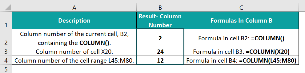
The above table shows the COLUMN function with example scenarios. In the target cell B2, the COLUMN() does not take any argument as input. Thus, it returns the column number of the current cell, B2, 2. In the second target cell, the requirement is to determine the column number of cell X20. And so, the COLUMN() accepts X20 as the argument to return the column number, 24. And in row 4, the requirement is to display the column number of the cell range L45:M80. So, the function takes the given cell range as the input and returns the column number of the first column in the range L45:M80, 12.

What is COLUMN Function in Excel?

The COLUMN function in Excel returns the column number of a given cell reference. Thus, users can apply this function while performing calculations involving specific column numbers or locating the required column number in a massive Excel dataset.
The COLUMN() takes one optional argument, reference.
We can opt not to provide the reference argument to the COLUMN Excel function. Otherwise, it can be a cell or cell range reference.
We can achieve excellent outcomes using the COLUMN function with other inbuilt Excel functions, such as IF, MOD, and VLOOKUP.

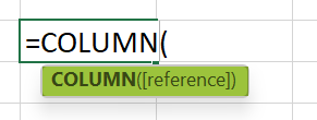
COLUMN() Excel Formula

The COLUMN formula in Excel is:

where,

reference: The cell or cell range for which we require the column number.

The argument reference in the COLUMN formula in Excel is optional.

Below are the critical aspects of the COLUMN function, we must know before using the COLUMN().

If we enter the COLUMN() in a cell without the reference argument, the function will return the column number of the cell where we entered the COLUMN().
Suppose the argument reference is a cell range, and we do not execute the COLUMN() as a horizontal array formula. Then the function output will be the number of the first column from the left.
Suppose we do not provide the reference argument, or it is a reference to a cell range, and we enter the COLUMN() as a horizontal array formula. Then the COLUMN function in Excel return value in each cell in the target horizontal array will be the column number of the respective cell reference.
We cannot supply the reference argument to the COLUMN() as references to multiple cell ranges.
If the argument reference is invalid, the COLUMN() returns the #NAME? error.

Excel VBA – All in One Courses Bundle (35+ Hours of Video Tutorials)

If you want to learn Excel and VBA professionally, then Excel VBA All in One Courses Bundle (35+ hours) is the perfect solution. Whether you’re a beginner or an experienced user, this bundle covers it all – from Basic Excel to Advanced Excel, Macros, Power Query, and VBA.

Start Learning Now

How To Use COLUMN Excel Function?

The steps to use the COLUMN function in Excel are:

First, confirm if the reference argument is the cell or cell range for which we require the column number.
Next, select the target cell and enter the COLUMN function.
Finally, press Enter to view the desired column number.

Let us understand the steps mentioned above to apply the COLUMN function in Excel with example.

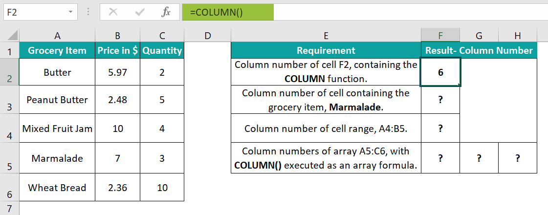
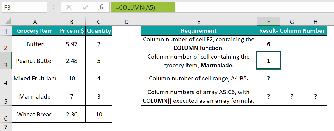
The first table in the below image contains a grocery item list. And the second table has the requirements for showing specific column numbers in target cells F2:F5 and G5:H5 from the first table.

We can get the required outcome using COLUMN function in Excel in the target cells, and the steps are:

Select the target cell F2, enter the COLUMN() without the argument reference, and press Enter.

As we did not supply the argument reference value to the COLUMN(), the function return value is the column number of the cell containing the COLUMN function, 6.
Select the target cell F3, enter the following COLUMN(), and press Enter.

=COLUMN(A5)

The specific grocery item, Marmalade, is in cell A5. Thus, the argument reference value in the COLUMN() in the target cell F3 is A5. So, the COLUMN function in Excel return value, in this case, is 1, the number of column A.

Alternatively, we can select the target cell F3 and click Formulas → Lookup & Reference → COLUMN to open the Function Arguments window.

Enter the reference argument value, A5, in the Function Arguments window.

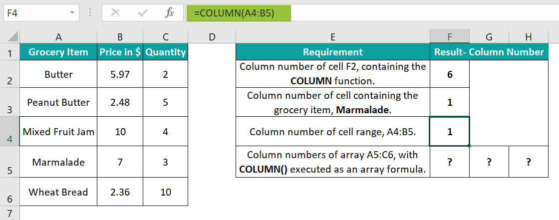
And once we click OK in the Function Arguments window, the required column number, 1, gets displayed in cell F3.
Select the target cell F4, enter the following COLUMN(), and press Enter.

=COLUMN(A4:B5)

As the requirement is to display the column number of the cell range, A4:B5, the COLUMN() argument is A4:B5. And since we do not execute the function as an array formula, it returns the number of the leftmost column in the range, 1.
Select the target cells F5:H5, enter the following COLUMN() in the curly brackets and then execute the function as an array formula using the keys Ctrl + Shift + Enter.

{=COLUMN(A5:C6)}

Here again, the reference argument is a cell range, A5:C6. But the requirement is to execute the COLUMN() as an array formula. So, we select the target array range, F5:H5, and apply the function as an array formula. And thus, the function returns the column numbers 1, 2, and 3 corresponding to the columns in the given range A5:C6.

Examples

Below are a few more examples to better understand the COLUMN function in Excel definition.

Example #1

Consider the below table. It shows monthly expenses details.

And suppose we need to add the miscellaneous expenses, provided in cell B6, to the monthly expenses, but every fourth month. And we have to show the revised expenses details in the target cell range B3:M3.

We can get the required data using the COLUMN with MOD and IF Excel functions in the target cells, and the steps are:

Step 1: To begin with, select the target cell B3, enter the below formula, and press Enter.

=IF(MOD(COLUMN(B2)-1,4)=0,$B$6+B2,B2)

Step 2: Next, drag the fill handle to the right to copy the formulas in range C3:M3.

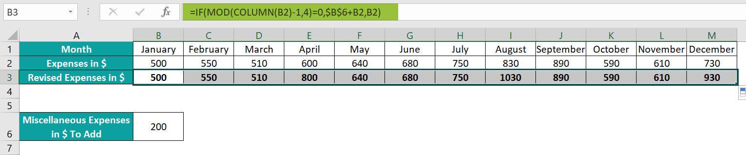
Thus, we get the revised expenses with the miscellaneous expenses added to April, August, and December expenses.

Let us see how the above formula works. Consider the expression in the target cell M3. First, the COLUMN function, COLUMN(M2), returns column number 13. So, the MOD() arguments are 12 and 4, making it return the value 0. Thus, the IF condition holds, and the miscellaneous expenses get added to the December expenses, making the revised December expenses $930.

Example #2

The first table in the following image shows ten test results.

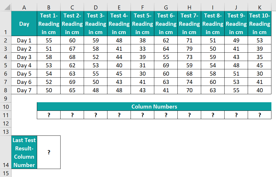
And suppose we require to determine the column number of each test and then find the last test column number to display in the target cell B14. Then, we can get the required output by applying the COLUMN and MAX function in Excel.

Step 1: First, select the cells B11:K11, enter the following COLUMN() in the curly brackets, and press Ctrl + Shift + Enter to execute the COLUMN function as an Excel array formula.

{=COLUMN(B1:K8)}

The COLUMN() updates the respective column numbers corresponding to the tests in cells B1:K8, in the cell range B11:K11.

Step 2: Next, select the target cell B14, enter the following MAX(), and press Enter.

=MAX(B11:K11)

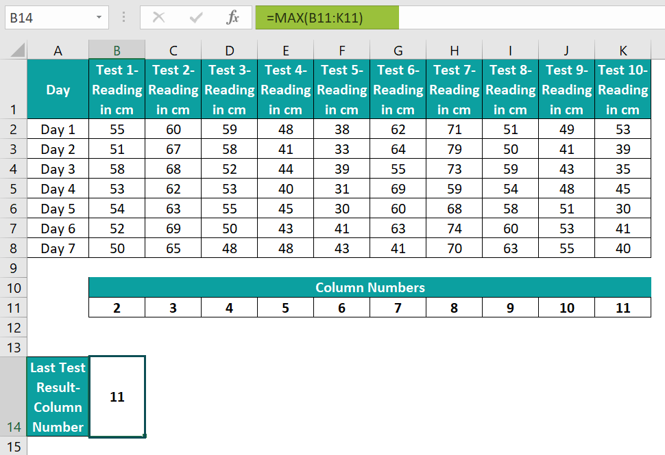
The MAX() returns the maximum number, 11, as the last test result column number.

Example #3

Let us see how to use the COLUMN function with VLOOKUP in Excel.

Suppose the first table in the below image contains employee details.

And we have to display details of employees with desktops based on the data in the first table in the target cells J3:K6.

Here is how we can use the VLOOKUP(), containing the COLUMN function in Excel, to achieve the required result.

Step 1: Select the target cell J3, enter the below formula, and press Enter.

=VLOOKUP(I3,A:B,COLUMN(B2),0)

Step 2: Drag the fill handle downwards to copy the formula in cell range J4:J6.

Step 3: Select the target cell K3, enter the below formula, and press Enter.

=VLOOKUP(I3,A:D,COLUMN(D2),0)

Step 4: Drag the fill handle downwards to copy the formula in cell range K4:K6.

Here is how the VLOOKUP formula containing the COLUMN() works. Let us consider the expression in cell K6. First, the COLUMN() inside the VLOOKUP() returns column number 4, based on the reference argument D5. Then the VLOOKUP() looks up the specific employee’s workstation ID in the first table to return the value ITIL_WS_053.

Important Things To Note

The COLUMN function in Excel argument cannot be a reference to multiple cell ranges. Also, if we supply an invalid argument value to the COLUMN(), the function returns the #NAME? error.
When we enter the COLUMN() in a cell without the reference argument, the function will return the column number of the cell where we entered the COLUMN().
Suppose the argument reference is a cell range. And we do not apply the COLUMN() as a horizontal array formula. Then the function output will be the number of the leftmost column.

Frequently Asked Questions (FAQs)

1. Where is the COLUMN function in Excel?

The COLUMN function is in the Formulas tab. Click Formulas → Lookup & Reference → COLUMN to access it.

2. Why is the COLUMN function not working in Excel?

The COLUMN function is not working in Excel, perhaps because of the below-mentioned reasons:
• The supplied reference argument is not a proper cell reference.
• You provided multiple references as the reference argument.
• The specific cell or cell range is invalid.

3. How to execute the COLUMN function in Excel VBA?

You can execute the COLUMN function in Excel VBA using the below steps. Let us see them with an example.

Suppose the given table is in the cell range D1:E6.

And to display the column numbers of the active cell and the last column with data, which are cell D1 and column E in the above example, in the target cells B1:B2. Then here is how we can use the COLUMN function in Excel VBA to update the target cells.

• Step 1: With the current worksheet open, press the keyboard shortcut keys Alt + F11 to open the VBA Editor window.

• Step 2: Next, choose the required VBAProject from the left menu and click Insert → Module to open the Module1 window.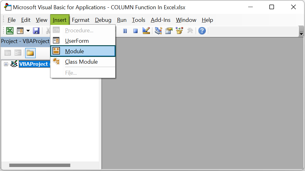

• Step 3: Enter the VBA code in the Module1 window to display the required column numbers in the target cells B1:B2.

Sub Column_fn()
Dim cn As Worksheet
Set cn = Worksheets(“FAQ 3”)
cn.Range(“B1”) = ActiveCell.Column
cn.Range(“B2”) = Cells(1, Columns.Count).End(xlToLeft).Column
End Sub

• Step 4: Click the Run Sub/UserForm icon in the menu to run the commands.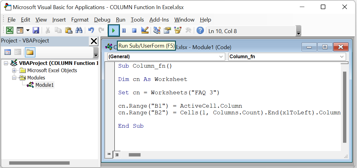

And once the commands get executed, the output in the active worksheet will be:

The active cell is D1. So, the column number of the D1 cell, 4, gets assigned to the target cell B1. And as column E is the last column with data, its column number, 5, gets populated in the target cell B2.

Download Template

This article must be helpful to understand the COLUMN Function In Excel, with its formula and examples. You can download the template here to use it instantly.

COLUMN Function In Excel Download

COLUMN Function In Excel