Excel Group Sum

What Is Group By Sum in Excel?

The Excel Group Sum calculates the total for the numeric values of a specific category. In a dataset, this feature first groups similar data values, such as month-wise, row-wise, or column-wise, and then returns the sum of their respective values.

To evaluate the Excel Group By Sum, we can use Excel functions such as SUBTOTAL(), SUM(), SUMIF(), SUMIFS(), etc., to find the total of the grouped category-wise data.

For example, the image below shows the values, and we will perform Excel Group Sum using the SUM function.

Enter the formula =SUM(1,2) in cell B2 to find the sum of values, and
Enter the formula =SUM(A2:A3) in cell B3 to find the sum of cells.
After entering each formula, press the “Enter” key.

The results in cells B2 & B3 are “3”, as shown above. Columns C & D are for our reference. When we add the cell references in excel or the cell values directly, either way, we get the same results.

What Is Excel Group By Sum?

The Excel Group Sum helps users to find the sum of the values that fulfill specific criteria.
We can calculate partial values such as row-wise, column-wise, month-wise, etc., using this option and find the sum of their respective values.
We can insert a criteria or a condition using Excel functions such as IF, SUMIF, SUMIFS, etc.
Since the functions related to Group Sum are inbuilt Excel functions, we can use them directly in the worksheet by grouping the cell values manually, or inserting the formulas from the “Formulas” tab, as we considered in the AutoSum examples.

How To Sum Values By Group In Excel?

We can Sum Values by Group in Excel in the following ways, namely,

Sum Group-Wise in Excel.
Combination Formula to Get Group-Wise Sum in Excel.

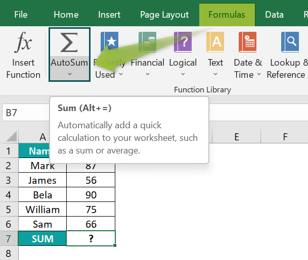
The below example depicts the scores of the students, and we will Sum them using the Excel Auto SUM Function, which is a part of Excel Group Sum.

In the table, the data is,

Column A contains the Name.
Column B contains the Scores.
Cell B7 contains the SUM.

How to Sum Values by Group in Excel - Basic Example

The steps to calculate the sum total using the Group by SUM in Excel are as follows:

Select cell B7 → go to the “Formulas” tab → go to the “Function Library” group → click the “AutoSum” option, as shown below.
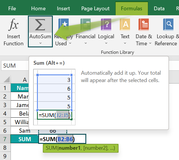
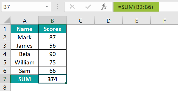
The complete formula that automatically appears the moment we click the AutoSum button is =SUM (B2:B6) in cell B7, as shown below.
Immediately press the “Enter” key. The result is “374”, as shown below.

Excel VBA – All in One Courses Bundle (35+ Hours of Video Tutorials)

If you want to learn Excel and VBA professionally, then Excel VBA All in One Courses Bundle (35+ hours) is the perfect solution. Whether you’re a beginner or an experienced user, this bundle covers it all – from Basic Excel to Advanced Excel, Macros, Power Query, and VBA.

Start Learning Now

Examples

We will consider some scenarios using the Excel Group Sum examples.

Example #1 – Sum Group-Wise in Excel

The succeeding example depicts the items, and we will Sum Group-Wise using the Excel SUM function.

In the table, the data is,

Column A contains the Items Group.
Column B contains the Items.
Column C contains the Price.
Column D contains the SUM.

Group Sum in Excel - Example 1 - Sum Group-Wise in Excel

The procedure to evaluate the values using the Excel SUM Function is,

Enter the formulas as follows:

=SUM(C2:C4) in cell D4,
=SUM(C5:C7) in cell D7, and
=SUM(C8:C10) in cell D10.
After entering each formula, press the “Enter” key.

Example 1 - Sum Group-Wise in Excel - Step 1

The results in cells D4, D7, and D10 are “400”, “310”, and “220”, respectively, as shown above.

Example #2 – Combination Formula to Get Group-Wise Sum in Excel

The succeeding example depicts the company’s monthly sales for two cities, and we will Combine Formula to get Group-Wise Sum using the Excel IF and SUMIF Functions.

In the table, the data is,

Column A contains the City.
Column B contains the Months.
Column C contains the Sales.
Column D contains the SUM.

Group Sum in Excel - Example 2 - Combination Formula to Get Group-Wise Sum in Excel

The steps to evaluate the values using the SUMIF and IF Excel Function are as follows:

Step 1: Select cell D2, enter the formula =IF(A2=A1, “ ”, SUMIF (A:A,A2,C:C)), and press “Enter”.

[Note:

The IF function’s ‘logical test condition’ value is A2:A1, i.e., the below cell value equals the above. The below cell has the same city name as the active cell in cell D2.
The SUMIF function’s ‘range’ value is A:A, i.e., Column A, “criteria” value A2, i.e., equal to the city name, “sum range” value is C:C, i.e., range of which sum is to be calculated in cell D2.]

Example 2 - Combination Formula to Get Group-Wise Sum in Excel - Step 1

The result in cell D2 is “$9,72,384”, as shown above.

Step 2: Select cell D6, enter the formula =IF(A2=A1, “ ”, SUMIF (A:A,A6,C:C)), and press “Enter”.

[Note:

The IF function’s ‘logical test condition’ value is A6:A5, i.e., the below cell value equals the above. The below cell has the same city name as the active cell in cell D6.
The SUMIF function’s ‘range’ value is A:A, i.e., Column A, “criteria” value A6, i.e., equal to the city name, “sum range” value is C:C, i.e., range of which sum is to be calculated in cell D6.]

Example 2 - Combination Formula to Get Group-Wise Sum in Excel - Step 2

The result in cell D6 is “$1,10,31,256”, as shown above.

Explanation And Usage Of Excel Group Sum

Explanation of Group Sum

In a dataset, we must specify the numeric values that have to be added, they can either be cell references or cell values. The Excel Group Sum first groups similar data values, and then calculates the sum using the Excel formula.

Usage of Group Sum

It is used to add the selected numeric values as per the specified criteria or conditions and then finds their SUM.
It is also used to exclude the values that don’t fall under the given criteria.

Important Things To Note

The data should be sorted based on the target group.
The “#NAME?” errors occur when a formula name or the cell range is incorrectly entered.
The “#VALUE!” occurs when a formula references an unexpected data style.

Frequently Asked Questions (FAQs)

1. What is the Shortcut for Add SUM function?

The syntax of the SUM formula is =SUM(number), and the shortcut keys are “ALT + =” .
It will automatically add a SUM formula to the cell, & calculate the sum based on the selected cell values.

2. What is the SUM formula?

The Excel SUM formula is used to add and calculate the total for the selected numerical values, cell values, ranges of values, or a combination of n numbers. If the data is updated or modified within the selected cell range of the formula, the formula automatically recalculates the sum each time.

3. How to SUM rows?

We will consider an example to SUM rows.

The succeeding example depicts the company’s sales, income, and profit, and we will Sum them in a Row using the Excel Auto SUM Function.

In the table, the data is,
• Row 2 contains the ABC Company.
• Row 3 contains the Net Sales.
• Row 4 contains the Other Income.
• Row 5 contains the Profit.
• Column N contains the SUM.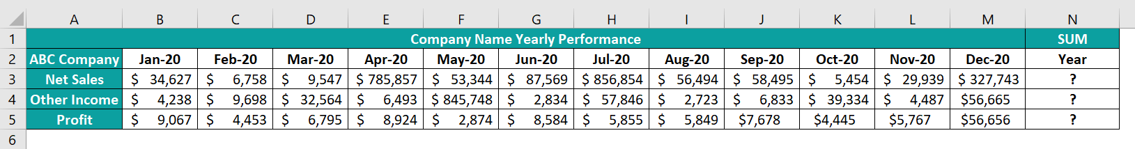

The steps to evaluate the values using the Excel SUM functions are as follows:

• Step 1: Select cell N3 → go to the “Formulas” tab → go to the “Function Library” group → click the “AutoSum” option.

The complete formula that automatically appears the moment we click the AutoSum button is =SUM (B3:M3) in cell B7, as shown below.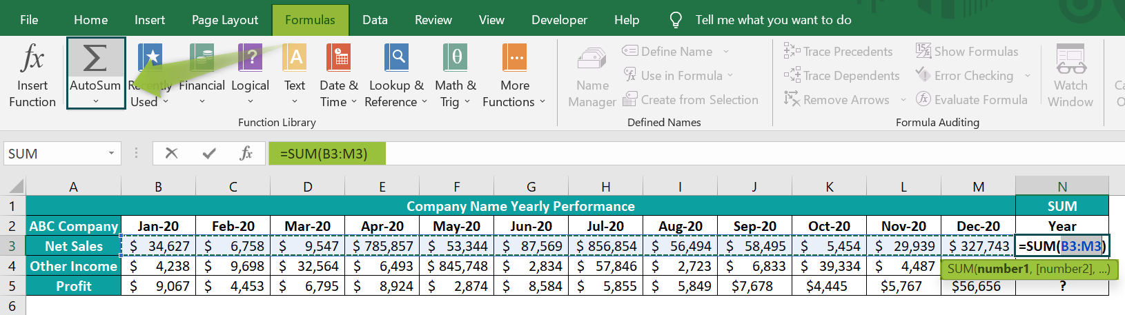

• Step 2: Now, press the “Enter” key. The result is “$23,12,681”, as shown below.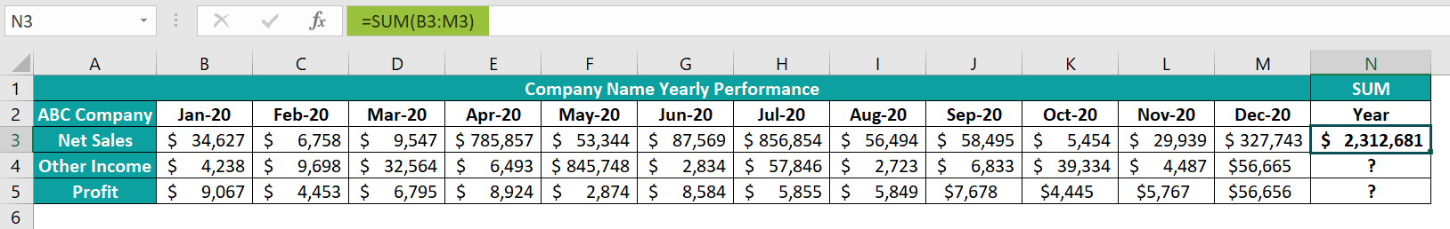

• Step 3: Drag the formula from cell N3 to N5 using the fill handle.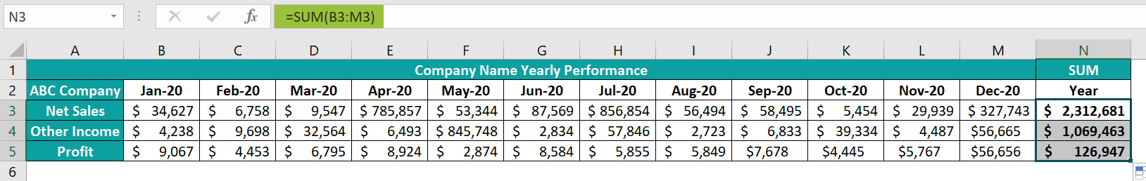

The output is shown above in cells N3 to N5, i.e., the sum of rows 3, 4, and 5.

Download Template

This article must help understand the Excel Group Sum’s formula and examples. You can download the template here to use it instantly.

Excel Group Sum Download

Excel Group Sum