
What Is MAXIFS Function In Excel?
The Excel MAXIFS Function returns the output as the maximum value depending on one or more than one conditions from the specified cells. The data is analyzed based on criteria. The MAXIFS Function is categorized under Statistical functions in the Function Library. The MAXIFS function was introduced in MS Excel 2019.
For example, suppose we have data and now, we will calculate the maximum value according to criteria using Excel MAXIFS Function.

The MAXIFS formula is entered in cell B7. So, the complete formula is =MAXIFS(B2:B6,A2:A6,”A”), and the result is returned as ‘50.’

Use this Excel MAXIFS Template to follow along with the examples in this article.
Download Excel TemplateKey Takeaways
- The MAXIFS function can fetch the highest value depending on a single or multiple criteria.
- MAXIFS is only present in Excel 2019 and Excel for Office 365
- Foe earlier Excel versions, we must use the MAX and IF functions with the criteria range.
- We must press the keys Control+Shift+Enter in Excel while entering an array formula.
- The #VALUE! error occurs when the size and shape of the “max_range” and “criteria_range” arguments aren’t the same.
MAXIFS() Excel Formula
The syntax of the Excel MAXIFS Formula is

- max_range: This shows the range of cells from the maximum value that will be determined.
- criteria_range1: These are the cells that are to be evaluated with the criteria.
- criteria1: This is the number, expression, or text that is to be evaluated as maximum.
Unlike other functions, all the arguments in the MAXIFS function are mandatory.
How To Use MAXIFS Excel Function?
1. Access From The Excel Ribbon
- Choose the empty cell which will contain the result.
- Go to the Formulas tab.
- Select the More Functions option from the drop-down menu.
- Select the Statistical option from the drop-down menu.
- Select MAXIFS from the drop-right menu.
- A window called Function Arguments appears.
- As the number of arguments, enter the value in the “max_range,” “criteria_range1,” & “criteria1.”
- Select OK.
2. Enter The Worksheet Manually
- Select an empty cell for the output.
- Type =MAXIFS( in the selected cell. Alternatively, type =M and double-click the MAXIFS function from the list of suggestions shown by Excel.
- Press Enter key.
Let us take an example to understand this function in detail –
The succeeding example depicts the marks of girls and boys, and we will calculate the maximum value according to the criteria using the Excel MAXIFS Function.
In the table,
- Column A contains the Gender.
- Column B contains the Marks.
- Cell B7 contains the Output.

The steps to evaluate the values by the Excel MAXIFS Function are as follows:
Step 1: First, select the cell where we will enter the formula and calculate the result. The selected cell, in this case, is cell B7.
Step 2: Next, we will enter the MAXIFS formula in cell B7.
Step 3: Then, enter the value of ‘max_range’ as B2:B6, i.e., the needed maximum range value.

Step 4: Now, enter the value of the ‘criteria_range1’ as “A2:A6,” i.e., the checked criteria range to perform the calculation.

Step 5: Also, enter the value of the ‘criteria1’ as “Boy,” i.e., the checked criteria to perform the calculation.
Step 6: So, the complete formula is =MAXIFS(B2:B6,A2:A6,”Boy”) in cell B7.

Step 7: After entering each value in the preceding step, press Enter key. The results in cell B7 are “98” in the image below.

Examples
Example #1
The succeeding example depicts the items and sales, and we will calculate the maximum value according to the criteria using the Excel MAXIFS Function.
In the table,
- Column A contains the Region.
- Column B contains the Item.
- Column C contains the Sales.
- Cell C10 contains the Output.

The steps to evaluate the values by the Excel MAXIFS Function are as follows:
Step 1: To begin with, select the cell where we will enter the formula and calculate the result. The selected cell, in this case, is cell C10.
Step 2: Next, we will enter the MAXIFS formula in cell C10.
Step 3: Then, enter the value of ‘max_range’ as B2:B9, i.e., the needed maximum range value.
Step 4: Also, enter the value of the ‘criteria_range1’ as “C2:C9,” i.e., the checked criteria range to perform the calculation.
Step 5: Now, enter the value of the ‘criteria1’ as “Books,” i.e., the checked criteria to perform the calculation.
Step 6: So, the complete formula is =MAXIFS(C2:C9,B2:B9,”Books”) in cell C10.
Step 7: Now, press Enter key.
The results in cell C10 are “$9,07,745” in the image below.

Likewise, we can use Excel MAXIFS function to find values.
Example #2
The succeeding example depicts the fruit cost of two years, and now, we will calculate the maximum value according to the criteria using the MAXIFS Function.
In the table,
- Column A contains the Fruits.
- Column B contains the Year.
- Cell C6 contains the Output.

The steps to evaluate the values by the Excel MAXIFS Function are as follows:
Step 1: First, select the cell where we will enter the formula and calculate the result. The selected cell, in this case, is cell C6.
Step 2: Next, we will enter the Excel MAXIFS formula in cell C6.
Step 3: Then, enter the value of ‘max_range’ as C2:C5, i.e., the needed maximum range value.
Step 4: Also, enter the value of the ‘criteria_range1’ as “A2:A5,” i.e., the checked criteria range to perform the calculation.
Step 5: Similarly, enter the value of the ‘criteria1’ as “Apple,” i.e., the checked criteria to perform the calculation.
Step 6: So, the complete formula is =MAXIFS(C2:C5,A2:A5,”Apple”) in cell C6.
Step 7: After entering each value in the preceding step, press Enter key. The results in cell C6 are “400” in the image below.

Similarly, we can use the function to find values.
Example #3
The succeeding example depicts the visitors according to the dates, and we will calculate the maximum value according to the criteria using the Excel MAXIFS Function.
In the table,
- Column A contains the Date.
- Column B contains the Visitors.
- Cell B10 contains the Output.

The steps to evaluate the values by the Excel MAXIFS Function are as follows:
Step 1: First, select the cell where we will enter the formula and calculate the result. The selected cell, in this case, is cell B10.
Step 2: Next, we will enter the MAXIFS formula in cell B10.
Step 3: Then, enter the value of ‘max_range’ as B2:B9, i.e., the needed maximum range value.
Step 4: Next, enter the value of the ‘criteria_range1’ as “A2:A9,” i.e., the checked criteria range to perform the calculation.
Step 5: Also, enter the value of the ‘criteria1’ as “>700,” i.e., the checked criteria to perform the calculation.
Step 6: So, the complete formula is =MAXIFS(B2:B9,A2:A9,”>700″) in cell B10.
Step 7: Finally, press Enter key. The results in cell B10 are “876” in the image below.

Likewise, using excel MAXIFS function, we can derive the desired output.
Important Things To Note
- The MAXIFS Function is used with the AND Excel function, which returns the maximum number that meets all specified conditions.
- The “max range” and “criteria ranges” arguments must have the same size and shape.
- The MAXIFS formula for multiple cells should be correctly entered.
- The MAXIFS Function is only available in MS Excel 2019 and Excel for Office 365. In earlier versions, this function is not available.
Frequently Asked Questions (FAQs)
The Excel MAXIFS Function returns the maximum value in a range that meets single or multiple criteria. The MAXIFS function is a built-in function in Excel that is categorized under a Statistical Function.
The logical operators like “>,<,>=,<=,<>,=”, and special characters like “* & ?” for partial matching.
The syntax of the MAXIFS function is as follows;
=MAXIFS(max_range,criteria_range,criteria)
The MAXIFS Function works in Excel by following the below steps;
1. First, select an empty cell for the output.
2. Next, type =MAXIFS( in the selected cell. Alternatively, type =M and double-click the MAXIFS function from the list of suggestions shown by Excel.
3. Then, press Enter key.
For example, suppose we have data and will calculate the maximum value according to criteria using Excel MAXIFS Function.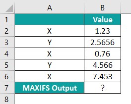
The steps to evaluate the values by the Excel MAXIFS Function are as follows:
Step 1: To begin with, select the cell where we will enter the formula and calculate the result. The selected cell, in this case, is cell B7.
Step 2: Next, we will enter the Excel MAXIFS formula in cell B7.
Step 3: Then, enter the value of ‘max_range’ as B2:B6, i.e., the needed maximum range value.
Step 4: Now, enter the value of the ‘criteria_range1’ as “A2:A6,” i.e., the checked criteria range to perform the calculation.
Step 5: Also, enter the value of the ‘criteria1’ as “Y,” i.e., the checked criteria to perform the calculation.
Step 6: So, the complete formula is =MAXIFS(B2:B6,A2:A6,”Y”) in cell B7.
Step 7: Next, press Enter key. The results in cell B7 are “4.566” in the image below.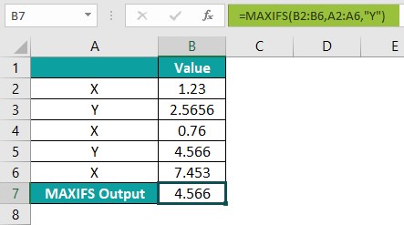
Similarly, we can use the function to find values.
We can insert MAXIFS Function using the following steps:
• First, choose the empty cell which will contain the result.
• Next, go to the Formulas tab and click it.
• Then, select the More Functions option from the drop-down menu.
• Now, select the Statistical option from the drop-down menu.
• Also, select MAXIFS from the drop-right menu.
• Meanwhile, a window called Function Arguments appears.
• As the number of arguments, enter the value in the “max_range,” “criteria_range1,” & “criteria1.”
• Select OK.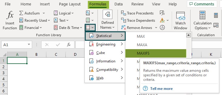
Use this Excel MAXIFS Template to follow along with the examples in this article.
Download Excel TemplateRecommended Articles
Continue with these related resources when you want the next practical step in this topic.
- IF Function In Excel
- Logical Operators in Excel
- Logical Test In Excel
- AND Function in Excel
- OR Function In Excel
Explore the full Excel Logical Functions guide or browse Excel Resources.