
What Is Find And Replace Feature In Excel?
The Find and Replace in Excel feature enables us to search and replace a data value with another value in one or more cells within a worksheet or workbook. The option is available under the Find & Select command in the Home tab.
Users can use the Find and Replace in Excel option to search a text string or numeric value by rows or columns and within comments, formulas, or values. And then replace the searched value with the required data.
Download FREE Find And Replace In Excel Template and Follow Along!Use this Find And Replace In Excel Template to follow along with the examples in this article.
Download Excel Template
For example, the table below lists a firm’s invoice numbers and products.

The requirement is to replace the “INVOICE” phrase in each invoice number with the “INV” phrase in cells A2:A11.
Then, we can perform multiple find and replace in Excel cell range A2:A11 using the Find and Replace option.

In the above multiple find and replace in Excel example, we choose the cell range A2:A11 and select the Replace option under the Find & Select feature in the Home tab.
The above action option gives us access to the Find and Replace window, where the Replace tab opens. Next, we enter the phrase we aim to replace, “INVOICE”, in the Find what field and the new phrase we wish to replace the existing phrase with, “INV”, in the Replace with field.
And then, on clicking the Replace All option, the phrase “INV” replaces the phrase “INVOICE” in all the chosen cells. Also, Excel shows a message box stating the total number of replacements, which is 10 in this example.
Finally, click OK in the message box to close it. After that, choose Close in the Find and Replace window to exit it and view the required output.
Key Takeaways
- The Find and Replace in Excel is a feature to locate and replace a value with the required data in a chosen dataset.
- Users can use the Find and Replace option to search for a specific value in a massive dataset and, if required, replace it with a value in one or more cells in one go.
- We can use the Find and Replace options under the Find & Select command in the Home tab to find and replace values in Excel.
- We can use wildcards in the Find and Replace feature to yield practical results.
How To Access The Find And Replace Feature Of Excel?
The top 3 methods to access the option to find and replace in Excel are as follows:
- Select the Home tab → Find & Select option down arrow → Find option. Otherwise, press Ctrl + F.
- Select the Home tab → Find & Select option down arrow → Replace option.
- Use the Find and Replace in Excel shortcut, Ctrl + H or Alt + H + FD + R.
The first method will give us access to the Find and Replace window, where the Find tab will be open. We can click the Replace tab to open it for using Find and Replace in Excel option.
On the other hand, the remaining methods will directly open the Replace tab of the Find and Replace window.
Examples
The following examples explain Find and Replace in Excel to use the option effectively.
Example #1 – Find A Partial Match In A Worksheet
The following image shows two tables listing the sales representatives at a firm and the monthly sales they generated.

The aim is to find cells containing Richard in the given dataset.
Since the sales representatives have first and last names, we can perform a partial match for the name Richard in the source dataset using Find and Replace in Excel option.
- Step 1: Click the triangle at the top-left corner of the workspace to select the entire sheet.
Next, select Home → Find & Select → Find.

The Find and Replace window opens, showing the Find tab.

- Step 2: Enter the search value “Richard” in the Find what field.

Clicking Find Next or pressing Enter will show the first cell containing the searched phrase in the selected sheet, with the finding process being a partial match and row-wise search.
Next, clicking Find Next or pressing Enter repeatedly will highlight the subsequent occurrences of the specified phrase, one cell at a time.


- Step 3: On the other hand, clicking Find All will list all the cells in the active sheet containing the searched phrase.


The result shows the workbook name, worksheet, cell addresses, and the values in the specified cells containing the searched phrase. Also, we can see the summary at the bottom-left corner of the Find and Replace window, showing the total cells identified containing the searched phrase in the worksheet.
We can then click the required entry from the list to navigate to the required cell containing the searched phrase in the dataset.
Furthermore, since the requirement is only to find a partial match for a value in the source dataset and not replace it, we use the Find tab in the Find and Replace window.
Example #2 – Find A Partial Match In A Workbook
The following example will explain Find and Replace in Excel workbook.
The below two images show two worksheets in a workbook, Richest US States and US States_Population.


The aim is to find a partial match for the US state of California in the active workbook.
Then, the steps are as follows:
- Step 1: Open the second worksheet, US States_Population, and choose Home → Find & Select → Find to access the Find tab in the Find and Replace window.

- Step 2: Enter “California” in the Find what field and click Options in the Find tab.

Excel will show more options to narrow down the search.

- Step 3: Click the Within field drop-down button and choose Workbook from the drop-down list.

Next, click Find All in the Find and Replace window.

Excel will summarize and list the cells containing data, partially matching the entered search term.
Furthermore, since the first sheet contains the first cell with the required partial match, the sheet becomes the active sheet, with the specific cell selected in the sheet.

Next, we can click the second entry in the search results to view the second cell in the second spreadsheet. So now, the second sheet becomes the current sheet, with the specific cell selected in the dataset.

Thus, the above examples show that the Find and Replace feature finds a match for the specified search value, even if there is data before or after the cited value within the cells. In such scenarios, the feature returns the entire strings in the cells containing the search value in the search results.
Example #3 – Find An Exact Match In A Workbook
The following image shows three worksheets in a workbook.
While each sheet contains the same employees, except the second sheet shows the first name of a few employees, the three sheets show their teams, IDs, and car park slots.


The requirement is to find the exact matches for the employee Jean Anderson in the workbook.
- Step 1: Open one of the worksheets in the workbook and choose Home → Find & Select → Find to access the Find tab of the Find and Replace window.

- Step 2: Enter the employee name Jean Anderson in the Find what field and click Options in the Find and Replace window.

We will see more options to narrow down the search.

- Step 3: Use the Within field drop-down button to access its drop-down list and choose Workbook.

Next, check the Match entire cell contents checkbox.

Finally, click Find All in the Find and Replace window.
Excel will summarize and list the cells containing an exact match for the entered search value.
Further, since the first sheet out of the three contains the first cell with the required exact match, the sheet becomes the active sheet, with the specific cell selected in the worksheet.

Next, click the second entry in the search results to view the second cell in the third spreadsheet. So now, the third sheet opens, with the specific cell selected in the dataset.

In the above example, the second sheet among the three sheets did not include Jean Anderson’s complete name. Hence, when the Find and Replace feature searched for an exact match in the workbook, it did not find one in the second sheet.
Thus, the search results show that only two cells contain data exactly matching the specified search value across the active workbook.
Example #4 – Replace The Range Reference Of A Formula
The first table in the image below lists fruits, their grades, and order data, with column C being a helper column containing unique key values based on the fruits and grades.
On the other hand, the second table lists the key values based on the fruits and grades in column G. Next, the second column, column H, contains the corresponding order status data, determined using the VLOOKUP Excel function based on the first table data.

However, the VLOOKUP() output in column H cells is an error value due to incorrect table_array and col_index_num values.
So, here is how to use the Find and Replace feature to correct the formulas and obtain the required output in column H.
- Step 1: Open the active sheet and choose Home → Find & Select → Replace.

[ Alternatively, use the Find and Replace in Excel shortcut, Ctrl + H.]
The Find and Replace window’s Replace tab opens.

- Step 2: Enter the VLOOKUP() formula applied in cell H2 in the Find what field in the Replace tab.

Next, enter the correct VLOOKUP(), with the updated table_array and col_index_num argument values, in the Replace with field in the Replace tab.

- Step 3: Press Replace All in the Find and Replace window.

Since the formula we aim to replace is in cell H2, it gets replaced with the correct expression and returns the required output in cell H2. Also, Excel shows a message box citing the total number of replacements.

Click OK to close the message box.

Next, click Close in the Find and Replace window to exit it.
- Step 4: Select cell H2 and update the formula in the remaining target cells using the Excel fill handle to achieve the desired outcome.

Example #5 – Replace The Existing Text To Make Two Strings Identical
The following image shows two sets of data.
The first one contains item codes, items and their order dates. The second one contains a list of item codes and their order dates updated using the VLOOKUP() based on the first dataset. Also, columns C and G have the same date formats.

However, the item codes in the second table are missing a hyphen, leading to the VLOOKUP(),resulting in error values in all the target cells.
So, here is how to use the Find and Replace in Excel option to overcome the issue.
- Step 1: Choose the cell range F2:F11 and press Ctrl + H to access the Replace tab of the Find and Replace window.
Next, please enter the phrase we aim to replace in the chosen cells in the Find what field.

Next, please enter the phrase we wish to replace the search value in the chosen dataset with in the Replace with field.
- Step 2: Press Replace All.

The correct phrase replaces the searched value in the chosen cells. Also, Excel shows a message box citing the total number of replacements done, which is 10 in this example.

- Step 3: Click OK to close the message box.

Finally, clicking Close in the Find and Replace window will close it, and we can view the required outcome.

Furthermore, once the item code strings in columns A and F become identical, the VLOOKUP() in the column G cells returns the correct output.
Example #6 – Replace The Old Formatting Of A Cell
The following image shows a dataset where the name Allen appears multiple times. Also, while three occurrences are in cells B2, C6, and D4, which have the same format, the fourth occurrence is in cell E3, which has a different format.

The aim is to replace cell E3 format with the format applied in the remaining three cells.
- Step 1: Choose the cell range B2:E6 and press Ctrl + H to access the Replace tab of the Find and Replace window.
Next, select Options in the Replace tab.

- Step 2: Excel will show a few more options to set the appropriate search and replace criteria.
Click the Format option drop-down button against the Find what field, and choose Format from the drop-down list.

The Find Format window will open, where we must select the Fill tab and choose the color set in cell E3 from the Background Color options.

Next, click OK.
Excel will show the chosen cell format in the preview in the Replace tab.

[ Alternatively, we can click the Format option drop-down button against the Find what field and choose Choose Format From Cell option from the drop-down list.

The cursor will appear as a fat white plus and eyedropper tool.

Select cell E3 to view the chosen cell format in the preview in the Replace tab.]
- Step 3: Click the Format option against the Replace with field and repeat step 2 to choose one of the three cells, say, the cell D4 format, to replace cell E3 format with it.


- Step 4: Click Replace All.

Cell E3 will now have the same format as the rest three cells containing the name Allen. Also, a message box will pop up, showing the total replacements done, which is 1 in this case.

Next, click OK to exit the message box.
Finally, click Close to close the Find and Replace window.

Thus, the final dataset will appear as shown below.

Example #7 – Find A Comment In A Worksheet
The following table lists two sets of values and the arithmetic operators to perform the required arithmetic operations with the values in the corresponding rows in column D.

Also, the column D cells contain comments, indicating the output of the corresponding arithmetic operations, Sum, Product, and Difference.
The requirement is to find the cells with the comment Sum in the source dataset.
- Step 1: Press Ctrl + F to access the Find and Replace window’s Find tab.
Next, enter the search value Sum in the Find what field and select Options in the Find tab.

We will see more options to help us narrow down the search.

- Step 2: Click the Look in field drop-down button to choose Comments from the drop-down list.

Finally, select Find All.

The search result will show the total count of cells and the references to the cells with the comments containing the search value Sum, which is 3 in this case.

Furthermore, the search action will be partially match-based.
Important Things To Note
- Choose the Find Next option in the Find tab in the Find and Replace window if we must search a value one cell at a time with the Find and Replace in Exceloption. Otherwise, use the Find All option to view all the cells containing the search value in one go.
- Select the Replace option in the Replace tab of the Find and Replace window if we must replace the search value one cell at a time in the required cell range. Otherwise, use the Replace All option to replace the search value with the required value in all the cells containing the search value in one go.
- The Find and Replace feature is case-insensitive. However, the feature offers an option, Match case, to perform a case-sensitive find and replace action.
Frequently Asked Questions (FAQs)
You can use wildcards in Excel Find and Replace option using the following steps, explained with an example.
The following table lists rhyming words in each cell.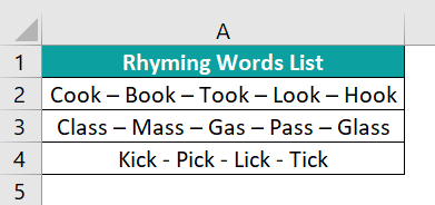
The requirement is to replace each word ending with “ook” with the word Shook. Then, the steps are as follows:
• Step 1: Press Ctrl + H to open the Find and Replace window’s Replace tab.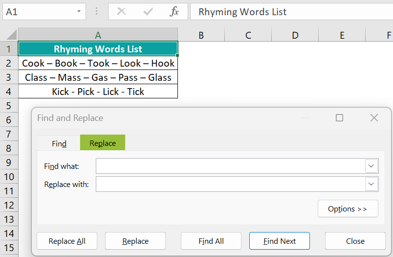
• Step 2: Since the source dataset contains rhyming words ending with “ook” and with one letter before the specified phrase, we shall use the wildcard character “?” in the search value.
So, the search value will be “?ook” in the Find what field in the Replace tab.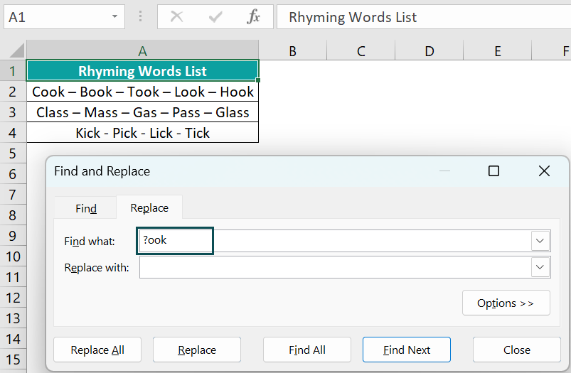
Next, enter the replacement value, “Shook”, in the Replace with field in the Replace tab.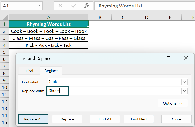
• Step 3: Select Replace All.
The required value, Shook, replaces all the words ending with “ook” and with one character before the phrase “ook”. Also, a message box shows the total replacements, which is 5 in this case, indicating the total words replaced in cell A2.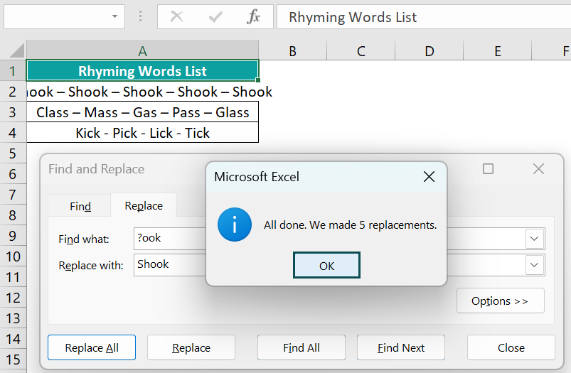
Click OK in the message box to exit it.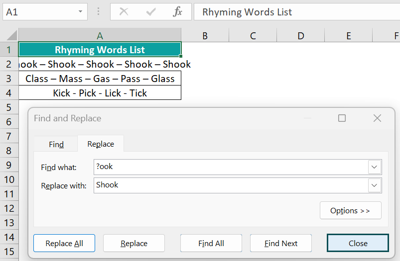
Finally, clicking Close will exit us from the Find and Replace window, and we can view the required output, as depicted below:
Find and Replace is not working in Excel, perhaps because of the following reasons:
• The active worksheet is password-protected.
• The active cells do not contain the search value.
• We use the Find and Replace feature when the search value is filtered and hidden in the dataset.
We can find and replace spaces in Excel using the following steps:
1) Select the required data range.
2) Press Ctrl + H to open the Replace tab of the Find and Replace dialog box.
3) Press the Spacebar in the Find what field and leave the Replace with field empty.
4) Click the Replace All button.
All the spaces in the chosen cells will get replaced, with a message box showing the total replacements.
Finally, click OK in the message box and Close in the Find and Replace window to view the required result.
Use this Find And Replace In Excel Template to follow along with the examples in this article.
Download Excel Template