What Is Format Cells in Google Sheets?
Formatting a Google sheet can help you organize and present data more effectively. Using the format cells in Google sheets feature, you can change the way your data looks, making your spreadsheet visually appealing and easier to understand. You can format cells by adjusting the text alignment, changing the date format, or adding color to your cells, in just a few clicks. There are different formatting options available in Google sheets. Here we give you a step-by-step guide that shows you how to format cells in Google Sheets.
In the example below, we have some data in a Google spreadsheet. We have formatted the cells by changing the font size and type as shown below. Thus, it is easy to format cells in Google sheets. Let us discuss on the different ways of implementing it in this article.

📥Download the ready-to-use Excel template to practice this tutorial yourself.
Format-Cells-in-Google-SheetsTable of contents
Key Takeaways
- When you format cells in Google sheets, you can change the way your data looks, making your spreadsheet easy to understand and functional.
- Cell formatting also makes the data more visually appealing.
- Use the “Format” tab and choose the type of formatting required under it.
- You can also directly format cells in Google sheets toolbar by selecting the range.
- Another way of formatting is by clicking “More formats” on the top menu which is a button that says “123.”
How to Format Cells in Google Sheets?
When we use Google sheets, formatting cells can help organize and understand different types of data. Be it financial data or even a sheet depicting weather patterns in a city, Google sheets can be formatted to understand the data clearly. Given below are the simple steps to format cells in Google sheets.
Step 1: Given below is some data. To format the cells, select range of cells by dragging your mouse over them.

Once you have selected the cells selected, the formatting options are available in the toolbar which can be seen above your data.
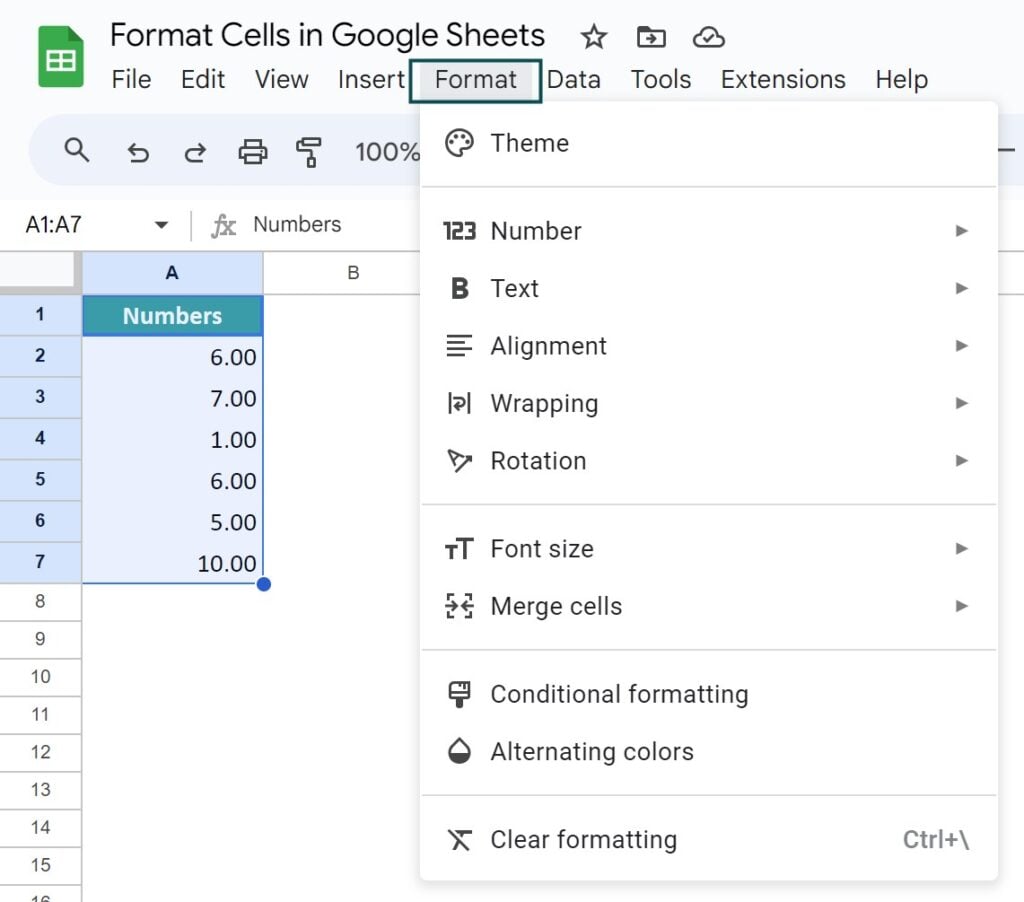
Step 2: Click on the “Format” option in the menu bar. This is the most valuable option which offers many types of formatting including text and number formatting, and cell color settings. This provides you with all necessary features to adjust your cell appearance.

Step 3: Select the desired formatting option from the dropdown menu. You can choose to format font, size, color, align text within the cell, or format numbers to display as date or fractions. In our example, lets align the text and display the numbers as currency.

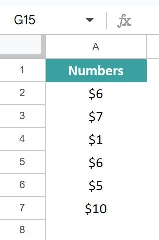
Step 4: As seen above, we are changing the alignment to Center, the result of which can be observed in the image below. Also, we have chosen the option “Number” followed by “Currency rounded” where we round off the currency to the nearest whole number.

Step 5: As you must have notices when we formatted the cells above, each formatting option comes with its set of options where you can fine-tune your choices. For example, you can choose a font style, select a background color, etc.
Step 6: Change the formatting and click “OK” or “Apply” to apply your formatting changes.

After completing these steps, your spreadsheet will carry the look you wanted and be more organized. It will help understand the data better, making the spreadsheet an ideal tool for data analysis.
Examples
Now that you have understood the basic rules on how to format cells, let us look at some different types of formatting which can be done with some interesting examples.
Example #1 – Format Date Cell
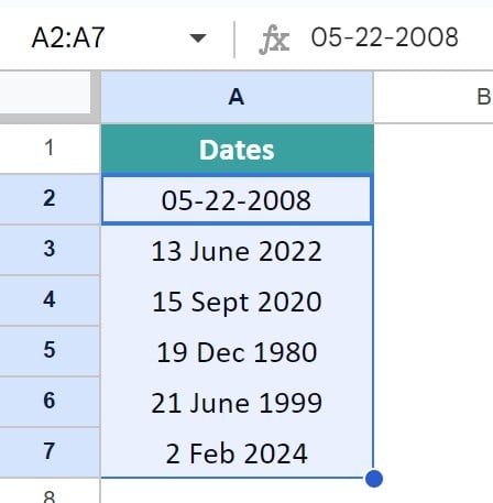
Below, we have some dates in a few cells.

Step 1: Select the cells containing the dates that you want to format.

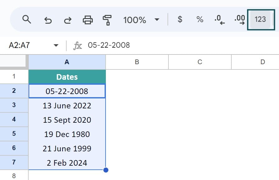
Step 2: Click “More formats” on the menu on top. This is a button which is displayed as “123.” Alternately, you can click “Format” – “Number.”

Choose the Google Sheets date format that you want. Google Sheets shows you a preview of each format. To look for further date formats, choose “Custom Date and time.”

You will be given a plethora of selections; choose the desired format and click “Apply.”

After following the steps above, the date format in the selected cells can be changed according to your preference.

Example #2 – Format Time Cell
Similar to how we changed the date format, let us try changing the time format as well. We have a list of time added in range C2 to C7.

Let us try to apply the time formatting for this range. After selecting this range, go to the “More Format” option in the tool bar.

Choose the “Custom Date and Time” option.

Choose the desired time option and see the formatting of the cells with time done instantly!

Example #3 – Format Date and Time Together
As seen in the above two examples, we have formatted the date and time separately. Let us merge the two cells together.
Step 1: Select the entire range from A1 to C7.

Step 2: We add the data in Column C in their corresponding row in Column A. The table is now as shown.

Step 3: To change the date-time format, go to Format – Form. Choose the “Custom Date and Time” option.

Step 4: Now, choose the desired format from the many options shown. Click Apply.

Step 5: You can observe how the date and time have changed in the Google sheet.

Example #4 – Positive and Negative Values
With the formatting options available in Google sheets, you can not only format date and time, but also format cells in number in Google sheets besides text in different ways. Let us look at an example. In the sheet below, we have the temperature in a city for the weeks ranging from Dec-Feb.

Step 1: To apply formatting and segregate the positive and negative temperatures, let us go to Format- Number and then scroll down to choose “Custom Number Format.”

Step 2: You get various options to separate the positive and negative numbers, as shown below.

Select the required option where you want to apply and click “Apply.”

Step 3: Check the segregation of the positive and negative values according to the format specified(negative numbers in brackets in red).

Example #5 – Add Suffix Words to Numbers
In this example, let us look at how to add suffixes to numbers in Google sheets. Adding suffixes and prefixes is a very useful format option available as we may have to give the units of data in many cases.
Below we have the weight of some people measured at a gym.

Step 1: It is hard to distinguish what the numbers represent without suitable suffixes. To add proper suffixes, first select the range of weight from B2 to B8. Then, go to “More Formats.” From there, choose “Custom Number Format.”

Step 2: In the pop-up, type the following in the in the Custom Number Format box.
## kg
Here, # represents any number present in the range. You can observe that Google Sheets gives you a preview of how the data looks like.

Step 3: Click Apply. The prefix is added to the range.

Example #6 – Using Format Painter
Format Painter in Google Sheets helps you copy the formatting on one cell/range to other cells without worrying about typing out the conditions/formula again. Let us look at our previous gym example and see how it can be applied. Three new members join the gym, and their weights are calculated.

Step 1: As you must have noticed, we had only specified the range up to B8. So, the suffix of kg is not applied to these values. We will show you how to apply it to the new range, i.e., B9 to B11.
Select the range B2 to B8 and click on “Paint Format,” the paint icon.

Step 2: Now, select the range from B9 till anywhere you want. Click on the range. The formatting is immediately applied to the selected range as shown below. Thus, copying the formatting and applying it to another range is very easy!

Important Things To Note
- Use the “Paint Format” tool in the toolbar if you wish to copy formatting from one cell and apply it to other cells.
- Google Sheets allows you to set up rules to format your cell depending on the formatting of another cell.
- To view different formatting options, once you have selected the cells, you’ll notice that the formatting options become available in the toolbar and are visible to you.
- When custom-formatting cells, you can format for positive and negative number under Number formatting.
Frequently Asked Questions (FAQs)
When you have cells containing numbers and wish to format them as currency or dates, you follow these simple steps.
Select the cells you wish to format.
Click the “Format” tab and click on Number.
Choose the desired format (e.g., currency, date).
The different types of format cells formatting in Google Sheets available include:
Font Formatting: Here, we can change the font size, color, and type for the sired cells. You can also highlight specific cells by adjusting font properties.
Alignment: You can change how you align text within cells(left, center, or right).
Number Formatting: You can format the given numbers based on your requirement as dates, currency, percentages, or decimals.
Besides this, the other forms of formatting include formatting the borders of cells, rows, and columns and finally, conditional formatting, where you can change cell formatting based on specific conditions.
Select the cell(s) whose formatting you wish to clear and go to Format -> Clear formatting. You can also use the shortcut key, Ctrl + \.
Applying alternating colors in Google Sheets helps understand the data better for easier scanning. It visually segments rows and uses the technique of formatting style and color to distinguish every other row within the specified data range. To apply alternating colors,
Highlight the desired range.
Click on “Format” > “Alternating colors.”
Select a scheme or customize your own.
Download Template
📥Download the ready-to-use Excel template to practice this tutorial yourself.
Format-Cells-in-Google-SheetsRecommended Articles
Guide to What is the Format Cells in Google Sheets. We explain how to use Format Cells in Google Sheets with examples. You can learn more from the following articles –

Leave a Reply