
What Is NA In Google Sheets?
The Not Available or the NA Google Sheets is a powerful tool that allows professionals to handle missing or invalid data effectively. By using the NA in Google Sheets, users can mark cells as not applicable or display an error value for data that is unavailable. This provides clarity and transparency in data analysis while ensuring accurate calculations.
With its ability to integrate seamlessly with other functions and formulas, the Google Sheets NA function proves to be invaluable in complex spreadsheets and financial models. It enables professionals to tackle issues related to missing values without compromising the integrity of their work. Furthermore, the flexibility of the NA function allows users to customize its behaviour based on specific requirements, making it a versatile solution for a wide range of data management scenarios.
Use this NA Google Sheets Template to follow along with the examples in this article.
Download Excel TemplateFor example, select cell A1, enter the formula =NA() and press “Enter”.

The output cell displays the “#N/A”, as shown above.
Key Takeaways
- NA Google Sheets enables professionals to handle errors smoothly, maintain data integrity, and streamline their workflow efficiently.
- The function can be used as a placeholder for cells with blank or unexpected values in formulas. This flexibility ensures that worksheets remain functional and accurate even when dealing with incomplete data sets or unforeseen circumstances.
- It simplifies the complex calculations involved in determining NA by providing a user-friendly interface and pre-built formulas. This software allows users to input parameters such as refractive index and focal length, and it instantly computes the numerical aperture.
- NA Google Sheets can generate comprehensive reports and graphs, making it invaluable for analyzing different optical systems and optimizing their efficiency.
Syntax
The syntax of the NA function in Google Sheets is,

The Google Sheets NA function does not require any arguments.
How To Use NA In Google Sheets? (With Steps)
We can use the AND In Google Sheets in 2 ways, namely,
- Access from the Google Sheets ribbon.
- Enter in the worksheet manually.
Method #1 – Access from the Google Sheets Ribbon 🡢
Choose an empty cell for the output 🡢 select the “Insert” tab 🡢 click the “Function” option right arrow 🡢 click the “Info” option right arrow 🡢 select the “NA” function, as shown below.

The “NA” formulaappears, as shown below. There is no need to enter any argument values, just press “Enter”.

Method #2 – Enter in the Worksheet Manually 🡢
- Select an empty cell for the output.
- Type =NA( in the cell. [Alternatively, type =N or =NA and double-click the NA function from the Google Sheets suggestions.]
- Close the brackets and press “Enter” as the function does not take or need any arguments.
Examples
Let us consider some examples to understand the NA Google Sheets function better.
Example #1
The table below consists of some units and its cost. We will calculate the total cost and check for NA Google Sheets error.

The steps to calculate the total cost are as follows:
Step 1: Select cell C2 and enter the formula =IF(A2=””,NA(),A2*B2)

Step 2: Press “Enter”. We get the output as “50”, as shown below.

Step 3: Drag the formula from cell C2 to C5 using the fill handle. The results are shown below. Please note that cell C4 has returned the #NA error.

Example #2
We will check for NA error in the table below which consist of Value 1 and Value 2. Create another table as shown in cells D1:E2 to use the VLOOKUP.

The steps to utilize the NA error using the VLOOKUP function in Google Sheets are as follows:
Step 1: Select cell E2 and enter the formula =VLOOKUP(D2,A1:B5,2,0)

Step 2: Press “Enter”. We see that the calculated result is #NA error because the looked-up value does not exist, as shown below.

Example #3
We will check for NA error in the table below which consist of Fruits andits price. Create another table as shown in cells F1:G3 to use the VLOOKUP.

The steps to utilize the NA error using the VLOOKUP function in Google Sheets are as follows:
Step 1: Select cell G2 and enter the formula =VLOOKUP(F2,A1:B6,2,0)

Step 2: Press “Enter” and drag the formula from cell G2 to G3 using the fill handle. We see that the calculated result is #NA error because the looked-up values do not exist, as shown below.

Example #4
The table below consists of some random numeric values where we will aplly a formula to increase the selected value by 10. Let us learn how to use NA Google Sheets.

The steps to perform the required calculation are as follows:
Step 1: Select cell B2 and enter the formula =IF(A2=””,NA(),A2+10) where the formula IF is incorporating the NA function, as shown below.

Step 2: Press “Enter” and drag the formula form cell B2 to B6 using the fill handle. The output is shown below and please note the cell C4 returns a #NA error.

How to Replace #N/A Values in Google Sheets?
We can replace #N/A Values in Google Sheets with 0 or blank using the IFERROR() formula.
Let us consider the Example 2’s output data as shown below.

- Now, enter the existing formula in cell E2 within the =IFERROR(), as shown below. So that the formula becomes =iferror(VLOOKUP(D2,A1:B5,2,0)) and the cell E2 instead of displaying “#NA” error has replaced it with blank cell.

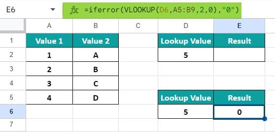
- We can also replace the NA error cell with zero. For that, create another table in cells D5:E6, just like the D1:E2 table. Now, select cell E6 and enter the new =IFERROR() formula as =iferror(VLOOKUP(D2,A1:B5,2,0),”0″) and the cell E6 instead of displaying “#NA” error or blank cell, has replaced it with 0, as shown below.
How To Remove #N/A in Google Sheets?
We can remove the #N/A in Google Sheets using the IFNA function.
Let us consider the Example 2’s output data as shown below.

Now, enter the existing formula in cell E2 within the =IFNA(), as shown below. So that the formula becomes =ifna(VLOOKUP(D2,A1:B5,2,0)) and the cell E2 instead of displaying “#NA” error will remove the error, as shown below.

Important Things To Note
- The NA function can be combined with other functions, such as VLOOKUP or IFERROR, to create more sophisticated formulas. By using these combinations, users can design complex algorithms that automatically skip or replace erroneous or absent values, improving the overall efficiency and reliability of their spreadsheet models.
- The main features of the NA function empower professionals to confidently work with data sets, knowing they have reliable methods for handling missing information.
Frequently Asked Questions (FAQs)
The NA function in Google Sheets is a valuable tool that allows users to identify and handle missing or unavailable data within their spreadsheets. One of the main features of this function is its ability to return the #N/A error value, which indicates that a particular cell does not contain valid information. This makes it easier for analysts and researchers to pinpoint and address any missing data points quickly, ensuring the accuracy and integrity of their calculations.
We often forget in which category a function falls, here, the “NA” function. Then, we can insert the function as follows:
Choose an empty cell 🡢 select the “Insert” tab 🡢 click the “Function” option right arrow 🡢 click the “All” option right arrow 🡢 select the “NA” function, as shown below.
However, as always, entering the function manually is the best way to avoid confusion.
Alternatively, we can find the Functions icon to insert the NA function by following the path shown below.
• Choose an empty cell 🡢 click the “More” option represented by the three vertical dots at the end of the toolbar, as shown below.
• A list of icons appears when we click the “More” option. Here, click the “Functions” icon, as shown below.
• Here, click the “Functions” option 🡢 click the “All” option right arrow 🡢 select the “NA” function, as shown below.
• One limitation is the restricted compatibility of NA Google Sheets with other software programs.
• Additionally, NA Google Sheets lacks advanced imputation techniques for filling in missing values, offering only limited options such as mean substitution or removing incomplete cases.
Use this NA Google Sheets Template to follow along with the examples in this article.
Download Excel Template