
What Is TREND Function In Excel?
The TREND Function in Excel evaluates the Y values based on a trendline for given X values, and the trendline is calculated using the least squares method based on two data series. The TREND in Excel is a statistical function under the function library.
For example, consider the below table with values in column A. We need to use the below steps to obtain the result using TREND function.

Use this TREND Function in Excel Template to follow along with the examples in this article.
Download Excel TemplateFirst, select the cell to display the result. In this example, we have selected cell B2. Next, enter the TREND Excel formula in cell B2. The complete formula is =TREND(A2:A3). Then, press Enter key. We can clearly see that the function has returned the value as 2.

Now, we can either apply the function manually or use the AutoFill Excel option. Similarly, we can find the values based on trendline using TREND Function in Excel.
Key Takeaways
- The TREND function in Excel is used to find values based on the trendline.
- The TREND Excel formula is =TREND(known_ys,[known_xs],[new_xs],[const]) where known_ys is the only mandatory arguments.
- The “#VALUE!” error occurs when the given known values of X or Y are non-numeric, or the value of new X is non-numeric.
- The “#VALUE!” error occurs when the “const” argument is not a Boolean value, i.e., TRUE or FALSE.
- The “#REF!” error occurs when X and Y values are of different lengths.
TREND() Excel Formula
The syntax of the TREND Fomula in Excel is

where,
- known_ys: It is the mandatory argument and denotes the set of ‘y’ values in the relationship of; y = mx + b.
- known_xs: It is an optional argument, and it indicates the set of ‘x’ values, and the value should be the same length as the set of known_y’s.
- new_xs: It is also an optional argument, showing one or more arrays of numeric values representing the ‘new_xs’ value.
- Const: It is the optional argument, specifying the value of the constant b to be 0 or 1. If ‘const’ is TRUE or 1, b is calculated normally; if ‘const’ is FALSE or 0, b is calculated as the m-values are adjusted so that y = mx.
How To Use TREND Excel Function?
We can insert TREND Function in Excel using the following two methods.
Method #1 – Access From The Excel Ribbon
- Choose the empty cell which will contain the result.
- Go to the Formulas tab.
- Select the More Functions option from the drop-down menu.
- Select the Statistical option from the menu.
- Select TREND from the drop-down menu.

- A window called Function Arguments appears.
- As the number of arguments, enter the value in the known_ys, known_xs, new_xs, & const.
- Select OK.

Method #2 – Enter The Worksheet Manually
- Select an empty cell for the output.
- Type =TREND( in the selected cell. Alternatively, type =T and double-click the TREND function from the list of suggestions shown by Excel.
- Press the Enter key.
Basic Example
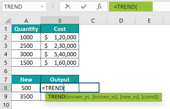
The below table shows products’ quantity and cost. We need to use the below steps to find the results using TREND Function.

The steps to evaluate the value with TREND Function in Excel are as follows:
- To begin with, select the cell where we will enter the formula and calculate the result. The selected cell, in this case, is cell B8.
- Next, we will enter the TREND function in excel formula in cell B8.
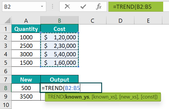
- Then, enter the value of ‘known_ys’ as B2:B5, i.e., the ‘y’ value.
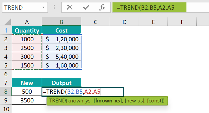
- Next, enter the value of ‘known_xs’ as A2:A5, i.e., the ‘x’ value.
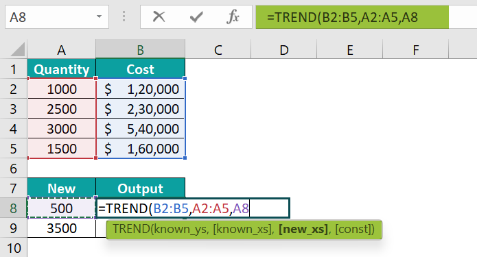
- Similarly, enter the value of ‘new_xs’ as A8, i.e., the new ‘x’ value.
- Now, enter the value of ‘const’ as TRUE, i.e., the const value.
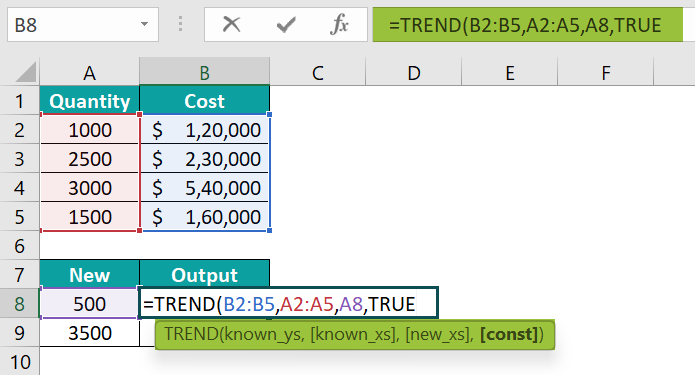
- So, the complete formula is =TREND(B2:B5,A2:A5,A8,TRUE) in cell B8.
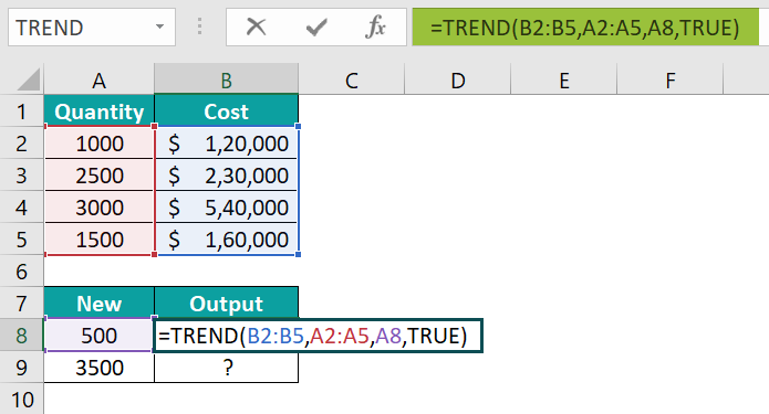
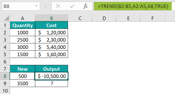
- Press Enter key. The function has returned the result in cell B8 as $-10,500.
- Next, enter the value of ‘const’ as FALSE, i.e., the const value.
- So, the complete formula is =TREND(B2:B5,A2:A5,A9,FALSE) in cell B9.
- Then, press Enter key.
So, the function has returned the result in cell B9 as $4,83,378.38.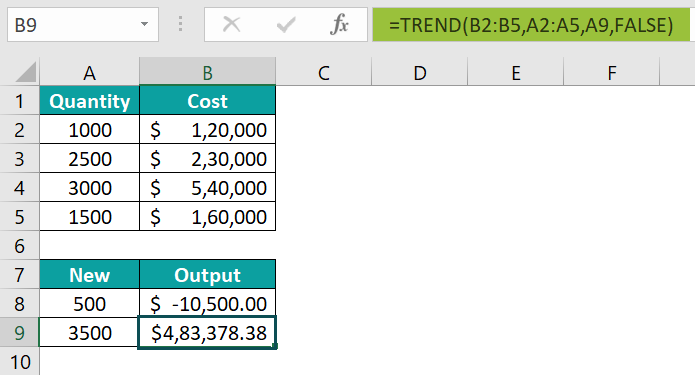
Similarly, we can use TREND Function in Excel to obtain the results.
Examples
Example #1
The below table shows date and sales data in columns A and B. We need to use the below steps to obtain the output using TREND Function in Excel.

The steps to evaluate the value using TREND Function are as follows:
- Step 1: To begin with, select the cell where we will enter the formula and calculate the result. The selected cell, in this case, is cell B7.
- Step 2: Next, we will enter the TREND formula in cell B7.
- Step 3: Then, enter the value of ‘known_ys’ as B2:B4, i.e., the ‘y’ value.
- Step 4: Now, enter the value of ‘known_xs’ as A2:A4, i.e., the ‘x’ value.
- Step 5: Similarly, enter the value of ‘new_xs’ as A7, i.e., the new ‘x’ value.
- Step 6: Finally, enter the value of ‘const’ as TRUE, i.e., the const value.
- Step 7: The complete formula is =TREND(B2:B4,A2:A4,A7,TRUE)in cell B7.
- Step 8: Then, press Enter key.
The function has returned the output in cell B7 as $77,82,307.81.

Likewise, we can use TREND function to find the output.
Example #2
The following table shows value x in column A and value y in column B. We need to use the below steps to find the output using TREND function in Excel.

The steps to evaluate the value by the TREND Function in Excel are as follows:
- Step 1: First, select the cell where we will enter the formula and calculate the result. The selected cell, in this case, is cell B8.
- Step 2: Next, we will enter the TREND formula in cell B8.
- Step 3: Then, enter the value of ‘known_ys’ as B2:B5, i.e., the ‘y’ value.
- Step 4: Now, enter the value of ‘known_xs’ as A2:A5, i.e., the ‘x’ value.
- Step 5: Also, enter the value of ‘new_xs’ as A8, i.e., the new ‘x’ value.
- Step 6: Similarly, enter the value of ‘const’ as FALSE, i.e., the const value.
- Step 7: So, the complete formula is =TREND(B2:B5,A2:A5,A8,FALSE)in cell B8.
- Step 8: Press Enter key.
The function has returned the result in cell B8 as 50.

Similarly, we can use TREND Function to fetch the output.
Example #3
The table below shows values x and y in columns A and B, respectively. We need to use the below steps to find the output using TREND Function in Excel.

The steps to evaluate the value by the TREND Function in Excel are as follows:
- Step 1: To begin with, select the cell where we will enter the formula and calculate the result. The selected cell, in this case, is cell B8.
- Step 2: Next, we will enter the TREND formula in cell B8.
- Step 3: Then, enter the value of ‘known_ys’ as B2:B5, i.e., the ‘y’ value.
- Step 4: Now, enter the value of ‘known_xs’ as A2:A5, i.e., the ‘x’ value in decimal.
- Step 5: Next, enter the value of ‘new_xs’ as A8, i.e., the new ‘x’ value in decimal.
- Step 6: Likewise, enter the value of ‘const’ as FALSE, i.e., the const value.
- Step 7: So, the complete formula is =TREND(B2:B5,A2:A5,A8,FALSE)in cell B8.
- Step 8: Press Enter key.
We can see that the function has returned the result in cell B8 as 45.669.

Thus, we can easily find the output from the given data using TREND Function in Excel.
Important Things To Note
- The TREND Function in Excel helps calculate an array of multiple values.
- The function can analyze revenue, cost, and investment.
- It is also used in investments to predict future shares.
- The existing data that contains the known values of X and Y needs to be linear data that, for the given values of X, the value of Y should fit the linear curve y=m*x + c.
- The TREND function helps the company to achieve its goals so that sales can be managed.
- The function is used as a real-time and time-based data analysis.
Frequently Asked Questions (FAQs)
The TREND Function in Excel is a least-squares method to match a data point in a linear trend for which it returns one or more numbers. The function predicts the value of ‘y’ from the given x and y values. The TREND function draws a line to show the relationship between the points for a given data set.
The syntax of the TREND Function in Excel is
=TREND(known_ys,[known_xs],[new_xs],[const])
The TREND function in Excel works by inserting it into a cell from the statistical functions list. The function is that multiple variables are used and could get mixed up while creating the formula manually by typing it in a cell. The TREND function works by the following steps:
Select the cell where the TREND function needs to appear. This would be in an area where the next trend point would appear.
• Type =TREND() in the selected cell. Alternatively, type =T and double-click the TREND function from the list of suggestions shown by Excel.
• Press Enter key.
For example, consider the below table with values in column A. We need to use the below steps to obtain the result using TREND function in Excel.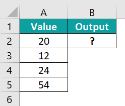
The steps used to find the result using TREND function in Excel are as follows:
• Step 1: Select the cell to display the result. In this example, we have selected cell B2.
• Step 2: Enter the TREND Excel formula in cell B2.
The complete formula is =TREND(A2:A5).
• Step 3: Press Enter key.
We can clearly see that the function has returned the value as 10.4.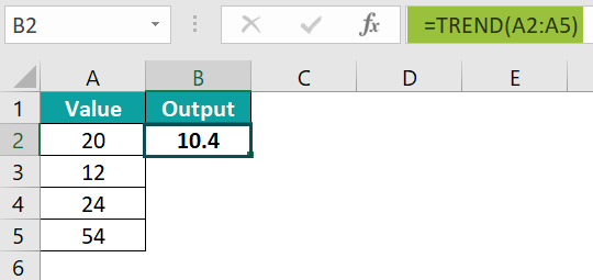
Similarly, we can find the values based on the trendline using TREND Function in Excel.
We can insert TREND Function in Excel using the following steps:
• Choose the empty cell which will contain the result.
• Go to the Formulas tab.
• Select the More Functions option from the drop-down menu.
• Select the Statistical option from the menu.
• Select TREND from the drop-down menu.
• A window called Function Arguments appears.
• As the number of arguments, enter the value in the known_ys, known_xs, new_xs, & const.
• Select OK.
Use this TREND Function in Excel Template to follow along with the examples in this article.
Download Excel TemplateRecommended Articles
Continue with these related resources when you want the next practical step in this topic.
- Statistics In Excel
- Descriptive Statistics in Excel
- Standard Deviation In Excel
- MEDIAN Excel Function
- MODE Excel Function
Explore the full Excel Statistical Functions guide or browse Excel Resources.