Data Model in Excel

What Is Data Model In Excel?

The Data model in Excel is a relationship or connection that is established between two or more tables based on the common column between those tables. Hence, when analyzing the data, the user can drag and drop the fields from other tables to get the information without formulas or calculated columns.

Data Model in Excel help us create a relationship between the fact table and dimension table to retrieve value from one to the other without actually applying any lookup functions.

What Is Data Model In Excel?

Data Model in Excel is creating a relationship between two or more tables based on the common column between tables.
When the data model is created between tables, we need to use any of the lookup functions to fetch the related values from dimension tables.
Either we can create data model in Excel first and then apply the pivot table, or we can insert pivot table and then create data modeling.
Data modeling creates a star schema where all the dimension tables filter the fact table.
Values in a dimension table should be unique, creating relationships between fact and dimension tables.

How To Create Data Model In Excel

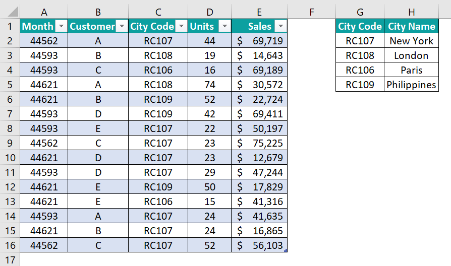
Let us first create Data Model in Excel exercise before moving into the advanced examples. We have the following two tables in Excel.

The first table, from A1:E16, is the fact table containing the monthly sales data (customer and city-wise).

However, in the first table, we have only the city code in column C and no city names in this table. In the second table we have city names based on each city code.

If we want to analyze the city-wise data, we need not have to insert the calculated column in the first table. Instead, we can create data model in excel between these two tables using the following steps.

Select any of the cell in the first table and convert them into Excel table format. Enter the shortcut keys Ctrl + T. The Create Table window pops up.
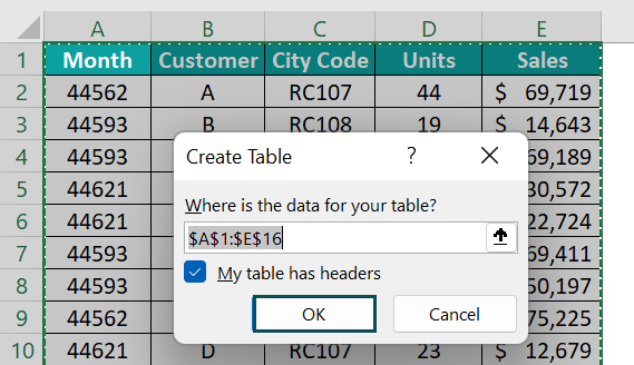
Make sure that My table has headers check box is selected because our table structure includes the headers, and we will get the following table structure.
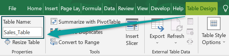
Select any cell in the table, and it will activate the Table Design tab in the ribbon. From this ribbon, give a name as Sales_Table.
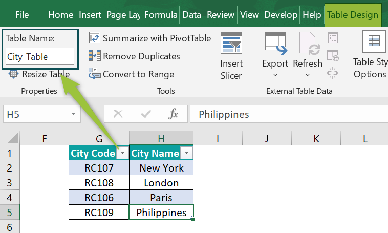
Repeat the same steps for the second table and name it as City_Table.
Now we have two Excel table structured formats. Now we need to create data model in excel between these two tables by creating a relationship.

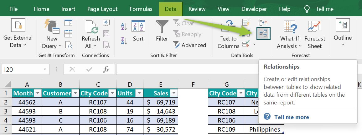
Go to the Data tab and click on the Relationships feature.
The Manage Relationships window opens up.

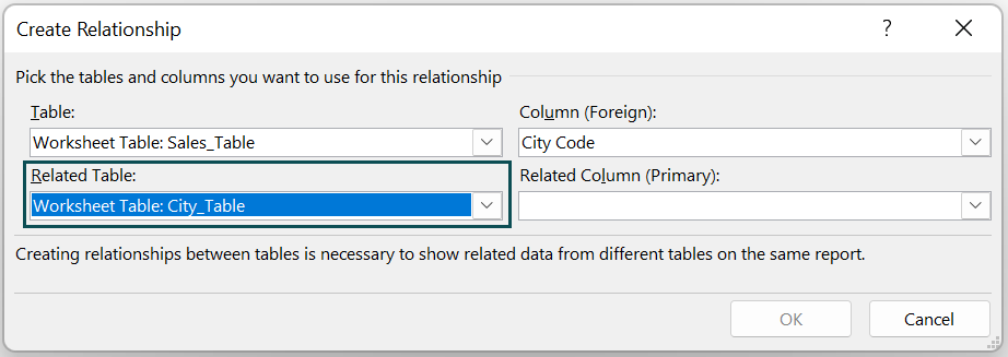
In this window, click on the New... button.
This will bring the following Create Relationship window. Choose the first table from the table drop-down list, i.e., Sales_Table.
From the selected table, we need to choose the column related to the second table, i.e., City Code.
Next, from the related table, choose City_Table.
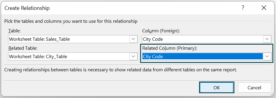
Next, from the city table, choose the column related to the Sales_Table, i.e., City Code column.
Click OK.
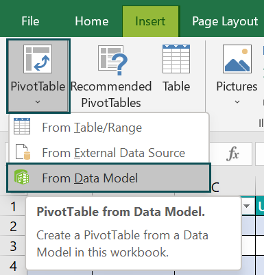
Now, we need to insert the pivot table. Go to the Insert tab, click on the PivotTable drop-down list, and choose the From Data Model option.

Note: We are using Office 2016 version Excel. If you are using any other version, it may vary.
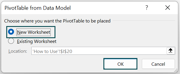
The PivotTable from Data Model window opens up. Choose New Worksheet option in this window.
Click OK, and we will get the new worksheet with the pivot table with a new data model.
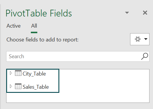
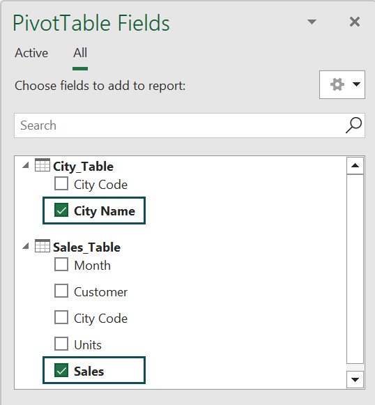
Drag and drop the city name from ‘City_Table’ and the sales column from ‘Sales_Table.’

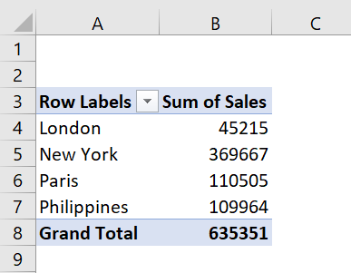
We will get the sales summary based on the city names.

Excel VBA – All in One Courses Bundle (35+ Hours of Video Tutorials)

If you want to learn Excel and VBA professionally, then Excel VBA All in One Courses Bundle (35+ hours) is the perfect solution. Whether you’re a beginner or an experienced user, this bundle covers it all – from Basic Excel to Advanced Excel, Macros, Power Query, and VBA.

Start Learning Now

Examples

Example #1 – Two Or More Tables Data Modeling

In the above example, we have seen how to create data modeling between 2 tables. Next, let us look at creating data modeling for more than three tables.

We have 3 tables in an Excel spreadsheet, as shown in the following image.

Orders_Table: The Order_Table contains order data for the region, product category, order date, and profit amount for each order.

Region_Table: The Region_Table contains information such as the managers for each region.

Returns_Table: The Returns_Table contains the order IDs and their status, and when we calculate the summary, we should exclude all the returned orders from the summary.

Let us create a model between three tables by creating a relationship between them. The following steps listed are:

Step 1: Convert all the tables into Excel Table format by pressing Ctrl + T.

Step 2: Give a name for the table as Orders_Table. Go to the Table Design tab and give a name, as shown in the following image.

Step 3: Repeat the same steps for the other two tables and name them Region_Table and Returns_Table.

Step 4: Once the Excel table format is applied to all the 3 tables, we need to establish a connection between these tables.

Go to the Data tab and click on the Relationship icon.

Step 5: This will bring the following Manage Relationships window. In this window, we can see all the existing relationships (the one we have earlier). Click on the New tab to create new relationship.

Step 6: After clicking on the new, we will get the following to create a relationship window. First, we will create a relationship between Orders_Table and Region_Table.

Choose the fact table, i.e., Orders_Table.

Step 7: From the Orders_Table, choose the Region column.

Step 8: Next, choose Region_Table from the Related Table drop-down table name.

Step 9: From Region_Table, choose the same column name we have chosen for the Orders_Table, i.e., Region column.

Step 10: Click on OK, and now the connection between Orders_Table and Region_Table is created. Now we can see the same in the manage relationship window.

In the same window, click on the New tab to a create relationship between Orders_Table and Returns_Table.

Step 11: Now choose the table as Orders_Table and the column name as Order ID.

Step 12: Similarly, choose Returns_Table from Related Table and the related column as Order ID.

Step 13: Click on OK, and we have a connection between all three tables.

Step 14: Now, go to the Insert tab, click on the PivotTable drop-down list and choose the option of From Data Model.

It will take the references from the existing data models we have created.

Step 15: Choose the option of New Worksheet or Existing Worksheet in the following window per the requirement.

New Worksheet: This will insert the pivot table in the new worksheet.

Existing Worksheet: This will insert the pivot table in the current worksheet.

Step 16: Drag and drop the columns from the required tables to create a summary report.

Data Model in Excel - Example 1 - Step 16

As shown in the above image, we have created a summary table of manager wise sales where the status is not returned.

In this summary Pivot table, we have Manager column from Region_Table, Status is from Returns_Table, and Sales is from Orders_Table.

Example #2 – Create Relationships After Creating A Pivot Table

We have seen the method to create data model in excel before applying the summary pivot table. We can also create data model in excel even after applying the pivot table.

Taking the same data from Example #1, let us apply the pivot table for the Orders_Table only.

In the above window, check the Add this data to the Data Model box.

Click on OK, which will allow us to play only with the Orders_Table.

However, we can still create a relationship between Region_Table and Returns_Table.

Select any cells in the pivot table inserted in the previous step, and we can see the Pivot Table Analyze tab in the ribbon.

Under this tab, we have the option of Relationships.

It will open up the manage relationship window like the following one.

Using the above window, we can create a relationship like how we have created in the previous examples.

After creating the relationships between tables, we can see all the data models we have created so far in the pivot table fields window.

As we can see, too many tables are not required.

To see the active pivot table data model, click on the Active option, showing only current pivot tables data modelling tables.

This way, we can create data modeling and play around with the data.

Important Things To Note

To create a data model, we need to have a common column between two or more tables.
There are two types of tables while creating data models, i.e., Fact Table and Dimension Table. The Fact Table contains all the facts about the data like sales, units, and profit, whereas Dimension table contains data related to dimensions like product info, customer info, region info, etc.,
To create relationships between tables, first, we need to convert the data range into Excel Table format.
If you use Excel 2106 and earlier versions, we need to check the box ‘Add this data to the Data Model’ while inserting the pivot table.
If you have multiple data models in your Excel file, when the pivot table is applied, it will show all the data model tables. However, we need to click on the ‘Active’ button to see only the current pivot table tables.

Frequently Asked Questions (FAQs)

1. How to Remove Table from Data Model in Excel?

To remove the table from the existing data model connection, we have to delete the relationship from the desired table.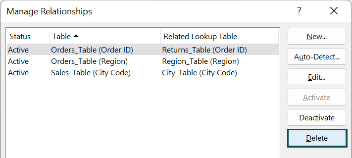

2. Where to find Data Model in Excel?

Data model is available under the Data tab in Excel as Relationship.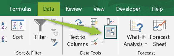

3. Why use Data Model in Excel?

Data model is so powerful that it eliminates the process of bringing in columns from other tables. So, for instance, if you want to bring the product name from the product table to the sales table based on the product ID, we can create Data Model in Excel and get the product name column directly from the product table in the pivot table summary.

4. Why can’t I add to Data Model in Excel?

If the file you are working on is a CSV file, then you cannot add it to the Data Model in Excel. Instead, you need to save the file as an xlsx file extension.

Download Template

This article must help understand the Data Model in Excel with its formula and examples. You can download the template here to use it instantly.

Data Model in Excel Download

Data Model in Excel