
What Is Data Table In Excel?
A Data Table in Excel helps study the variation in outputs resulting from a change in one or two inputs (or variables) of a formula. The two inputs can have as many possible values as desired. However, one cannot change more than two inputs of a formula. Data tables are used when different input and output combinations need to be examined in Excel.
For example, Mr. X wants to invest a monthly amount of $10,000 in a savings plan whose rate of interest (or ROI) is 10% per annum. He wants to know the return he will get when the rates vary from 10% to 20%. A data table (D4:E15) is created in the following image. Column E shows various future values (or returns) at different rates of interest (column D).

Use this Data Table in Excel Template to follow along with the examples in this article.
Download Excel TemplateKey Takeaways
- A Data Table of Excel allows analyzing the outputs and explore a range of possibilities resulting from a change in focus on only one or two variables..
- The outputs of the data table depend on the formula cell of the source dataset. Any changes to the formula cell cause the outputs to change automatically, provided the two are connected with a linked cell.
- The individual output cells of the data table cannot be edited or deleted as it uses array formulas for calculations.
Types of Data Tables in Excel
Data tables, Scenarios, and Goal Seek are parts of the What-If Analysis Excel tools. In a data table, the formula to be examined depends on several inputs.
There are two kinds of data tables in Excel. They are stated as follows:
- One-variable data table
- Two-variable data table
Let us discuss each type of data table one by one with the help of examples.
One-Variable Data Table
A one-variable data table helps study the impact on outputs resulting from a change in one input of the formula. One-variable data tables can be either row-oriented or column-oriented. In the former, the possible values assumed by an input are listed in a row, while in the latter; the possible values are listed in a column.
Let us understand this concept with an example.
Mr. A runs a textile business that has generated a revenue of $500,000 in the current year. The sales are assumed to grow by 10% in the subsequent year.
Create a one-variable data table when sales are forecasted to grow at 10%, 12%, 14%, 16%, 18%, and 20%. The data table should be row-oriented.

The steps to create a one-variable data table in Excel are listed as follows:
Step 1: Enter the following formula in cell B4.
“=(B2*B3)+B2”
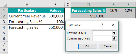
Press the “Enter” key and the output is $550,000. This figure represents the forecasted sales when the growth rate (or forecasted sales percentage) is 10%.

Step 2: Enter the possible values that the input (cell B3) can assume in the range E1:J1.

Step 3: Link cell D2 with the formula cell (B4). For linking, type “=B4” in cell D2 and press the “Enter” key.
When the possible input values are in a row, the cell immediately below and to the left of these values (cell D2) must be linked with the formula cell (cell B4). The linking of cells D2 with B4 ensures that any changes in the formula of the former cause the outputs to update automatically.
Note: When the data table is column-oriented, the cell immediately above and to the right of the possible input values must be linked with the formula cell.

Step 4: Select the entire range (D1:J2) of the data table. The selection should include the possible input values (E1:J1), the linked cell (D2), and the empty cells for the outputs (E2:J2).

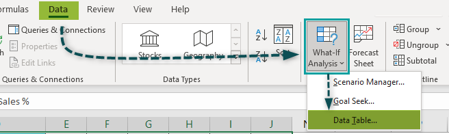
Step 5: Click the “What-If Analysis” drop-down (“data tools” group) from the Data tab of Excel. Select the option “data table.”
Step 6: The “data table” window opens, as shown in the following image.
Step 7: Select cell B3 as the “row input cell.” The reference $B$3 appears in this box. Since our one-variable data table is row-oriented, the “row input cell” is specified though the “column input cell” is left blank.
Note: In a column-oriented data table, the “row input cell” is left blank though the “column input cell” is supplied.

Step 8: Click “OK” in the “data table” window. The outputs are shown in the following image. Notice that the formula bar shows the formula “{=TABLE(B3,)}.”
Further, as the forecasted sales percentage (in E1:J1) increases, the amount of forecasted sales (in E2:J2) increases. Hence, we can analyze the variations in the outputs resulting from a change in one input, i.e., the growth rate (or forecasted sales percentage).
Note: Excel uses either the formula “=TABLE(row_input_cell,)” or “=TABLE(,column_input_cell)” to calculate the outputs of a one-variable data table. The former formula is used in a row-oriented data table, while the latter is used in a column-oriented data table.

Two-Variable Data Table
A two-variable data table helps study the impact on outputs resulting from a change in two inputs of the formula. A two-variable data table has two series (or lists) of possible values assumed by an input. One series is listed in a row while the other is listed in a column.
Let us understand this concept with an example.
There are two images titled “image 1” and “image 2.” The following information is given:
- “Image 1” shows that Mrs. D has invested $100,000 for 20 years at the rate of 10% per annum.
- “Image 2” shows the possible values in the ranges F2:K2 and E3:E11 that the ROI and the investment amount can assume.
Create a two-variable data table to observe the different future values (or returns) obtained by changing two inputs (ROI and investment amount).
Image 1

Image 2

The steps to create a two-variable data table in Excel are listed as follows:
Step 1: Enter the following formula in cell B5.
“=FV(B3,B4,-B2)”
Press the “Enter” key. The output is $5,727,500. This is the return that Mrs. D will get if she invests $100,000 at 10% for 20 years.
Note: The FV function returns the future value of an investment based on the supplied interest rate, investment amount, and time period.

Step 2: Link cell E2 with cell B5. By linking these cells, the outputs of the data table update with a change in the formula of cell B5.

Step 3: Select the range E2:K11. This is the range of the entire data table.

Step 4: Click “data table” from the “What-If Analysis” drop-down of the Data tab. The “data table” window opens.

Step 5: Select cells B3 and B2 in “row input cell” and “column input cell” respectively. This is because the different rates are in a row (F2:K2) while the investment amounts are in a column (E3:E11).

Step 6: Click “OK” in the “data table” window. The outputs are shown in the following image. Notice that Excel has used the formula “{=TABLE(B3,B2)}” in calculating the outputs.
From the data table, one can infer that the more the rate and the investment amount, the greater the future value (or return) earned by Mrs. D.
Note: In a two-variable data table, Excel uses the formula “=TABLE(row_input_cell,column_input_cell)” to calculate the outputs. So, it is essential to supply both “row input cell” and “column input cell” in a two-variable data table of Excel.

Examples
Example #1–Find The Affordable Payment Amount When The Loan Tenure Varies
Miss Amelia saves $50,000 per month from her current salary. She wants to take a personal loan of $1,500,000 at 10.5% per annum for 6 years.
Find the optimum tenure and the maximum monthly amount she can afford to pay on the loan if the years are varied from 2 to 6. Create a one-variable, column-oriented data table.

The steps to create a one-variable data table in Excel are listed as follows:
Step 1: Enter the following formula in cell B5.
“=PMT(B3/12,B4*12,-B2)”
Press the “Enter” key. The output is $28,168. This implies that if Miss Amelia opts for a six-year tenure, she will have to pay $28,168 on a monthly basis to settle the loan.
Note: The PMT function returns the amount to be paid on a loan based on the supplied interest rate, payment period, and borrowed amount.

Step 2: List the possible values assumed by the input “years” in column D. These are shown in the following image.

Step 3: Link cells E1 and B5 by entering “=B5” in the former.

Step 4: Select the range D1:E6 and open the “data table” window. For opening this window, select the option “data table” from the “What-If Analysis” drop-down of the Data tab.

Step 5: Enter the reference $B$4 as the “column input cell.” Omit the argument “row input cell” as this is a column-oriented data table.

Step 6: Click “OK” in the “data table” window. The outputs are shown in column E of the following image.
Hence, Miss Amelia must select the tenure of 3 years and monthly payment of $48,754. This is because this is the maximum amount she can pay, considering her monthly savings of $50,000.

Example #2–Find The Affordable Payment Amount When The Loan Tenure And Rate Of Interest Vary
Consider Miss Amelia of example #1 again. Assume that her loan amount ($1,500,000), interest rate (10.50%), and savings amount ($50,000) stay the same.
Further, she wants to know the maximum monthly amount she can afford to pay when the interest rate and time period vary. The possible values that these two inputs can assume are listed in the ranges F3:M3 and E4:E10 of the following image.
Create a two-variable data table of Excel. The value of cell B5 has been calculated by the formula “=PMT(B3/12,B4*12,-B2).”

The steps to create a two-variable data table in Excel are listed as follows:
Step 1: Link cell E3 with B5. For linking, enter the formula “=B5” in cell E3.

Step 2: Select the range E3:M10.

Step 3: Click the “data table” option from the “What-If Analysis” drop-down of the Data tab. The “data table” window opens in Excel.

Step 4: Select cell B3 as the “row input cell” and B4 as the “column input cell.” This is because these cells contain the inputs that can assume different values.

Step 5: Click “OK” in the “data table” window. The outputs are shown in the following image. Notice that the formula of the formula bar includes both the “row input cell” and the “column input cell.”
The range F4:M10 shows the different outputs when two inputs (interest rate and the number of years) are changed.

Step 6: Miss Amelia should choose a combination of 3 years and an interest rate of 10.5%. The monthly amount at the intersection of these two inputs is $48,754. This amount is the maximum that Miss Amelia can afford to pay for the loan, given her savings of $50,000.

Important Things To Note
The important points related to the data tables of Excel are listed as follows:
- A data table can be either one-variable or two-variable.
- A data table uses the TABLE array formula to calculate the outputs.
- One must specify the “row input cell” and/or the “column input cell” depending on whether the possible input values are in a row, column, or both. Moreover, the input cells should be on the same worksheet as the data table.
- The linked cell of the data table must contain a reference to the formula cell of the source dataset.
Frequently Asked Questions (FAQs)
In Excel, the “data table” option is under the “What-If Analysis” drop-down of the Data tab. This drop-down is in the “data tools” group.
Once the “data table” option is clicked, a “data table” window opens, as shown in the following image.
It is not possible to delete a single cell of an Excel data table. If one tries to delete a single cell, a message appears. This is shown in the following image.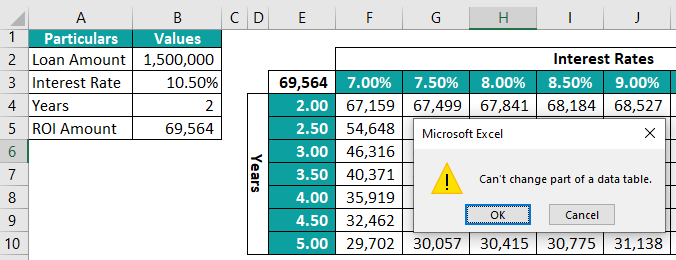
The steps to delete a data table (given in step 6 of example #2) in Excel are listed as follows:
a. Select either the entire range of the data table (E3:M10) or the output cells (F4:M10).
b. Press the “Delete” key.
It is not possible to edit the individual cells of a data table as they are part of an array. Therefore, to edit, one may delete the existing data table and create a new one.
A data table may not work in Excel for the following reasons:
a. The input cells and the data table may be located on different worksheets.
b. The specified references for the “row input cell” and/or the “column input cell” may be incorrect.
c. The sheet containing the data table may be protected. In this case, the data table is in a read-only mode. So, one should unprotect the sheet before working on the data table.
d. The empty range selected for outputs may contain a mix of locked and unlocked cells.
e. The linked cell may neither contain the formula whose outputs are to be studied nor the reference to the formula cell of the source dataset.
Use this Data Table in Excel Template to follow along with the examples in this article.
Download Excel Template