VLOOKUP With MATCH

What Is VLOOKUP With MATCH Function In Excel?

The VLOOKUP retrieves the values from the desired column based on the lookup_value provided. However, the VLOOKUP function requires the column index number from which column of the table array we need to retrieve the desired result, and this column index number is often static. Therefore, if any columns are added or deleted from the selected table array, we will get the #N/A error because of the static column index number provided.

The MATCH function will help us get the column index number to the VLOOKUP function dynamically based on the header of the column provided. This way, the VLOOKUP function always returns the correct value for the header provided.

What Is VLOOKUP With MATCH Function In Excel?

The VLOOKUP with MATCH always fetches the exact match from the desired columns, irrespective of the deletion or addition of columns.
The MATCH function will help us get the column index number to the VLOOKUP function dynamically based on the column’s header.
The MATCH function returns the position (row or column number) of the lookup_value in the given lookup_array.
For the MATCH function to return the position of the lookup_value, the order of the column doesn’t matter.

Problems With VLOOKUP

Let us consider the problems we encounter using the VLOOKUP function that accepts the static column index number.

Excel VBA – All in One Courses Bundle (35+ Hours of Video Tutorials)

If you want to learn Excel and VBA professionally, then Excel VBA All in One Courses Bundle (35+ hours) is the perfect solution. Whether you’re a beginner or an experienced user, this bundle covers it all – from Basic Excel to Advanced Excel, Macros, Power Query, and VBA.

Start Learning Now

Problem #1

For instance, look at the following VLOOKUP function in Excel.

In cell G2, we have applied the VLOOKUP function to get the employee salary based on the employee id. The column index number given is 3, i.e., the table array A2:D9 from the 3^rd column, from which we are retrieving the salary information.

Now, imagine that we remove the employee’s name column, i.e., column B, in the table array.

The output for the same formula gives us a different result.

The reason is when we removed the “Employee Name” column from the table array, every other column to the right of the deleted column shifted one column to the left, and their positions changed.

The “Salary” column becomes the 2^nd column, and the “Department” column becomes the 3^rd column. Since we have given a static column index number in the VLOOKUP function, it returns the value from the 3^rd column, i.e., the “Department” column.

This is the drawback of giving the static column index numbers to the VLOOKUP function that can be fixed using the VLOOKUP with MATCH excel function.

Problem #2

For instance, look at the following example of the VLOOKUP function.

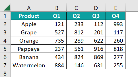
We have the product-wise quarterly number of units sold data in Excel.

From the above table, we will retrieve one of the product’s sales unit numbers like the following. We will retrieve the “Orange” product sales unit numbers.

The challenges are, first, the quarter numbers are not in order, and second, we need to apply VLOOKUP once (with references locked accordingly), and then keep changing the column numbers for the respective quarter column manually, which is time-consuming. To fix such issues, we use the MATCH function to retrieve the column numbers for each quarter dynamically.

VLOOKUP MATCH Formula

We are familiar with the VLOOKUP function. Let us look at the syntax of the MATCH function.

MATCH function → It will return the row/column number for the lookup_value in the lookup_array.

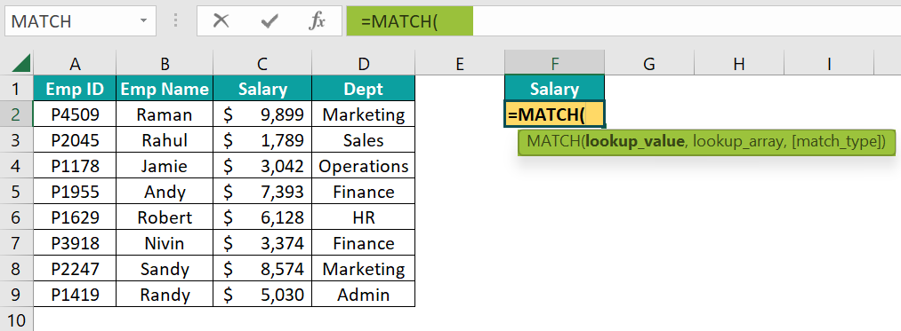
The syntax of the Match function is,

The arguments of the Match function are,

lookup_value: The value for which we find the row or column number.
lookup_array: The table area we find the row or column number for the desired lookup_value.
[match_type]: There are 3 matching types available as follows:
- 1: It will look for the largest value, either less than or equal to the lookup_value provided, and returns the approximate match. It requires the lookup_array to be arranged in ascending order (lower to higher or A to Z).
- 0: It will return the exact match to the lookup_value, irrespective of how the data is arranged or sorted.
- -1: This will search for the smallest value which is either greater than or equal to the lookup_value provided, and returns the approximate match. It requires the lookup_array to be arranged in descending order (higher to lower or Z to A).

Let us take a basic example to see its application.

First, let us understand how the MATCH function works.

For instance, look at the following data in Excel.

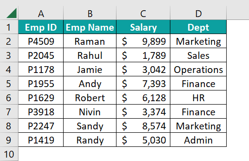
Now let us find the column number position for the column header “Salary”.

Enter the MATCH function in cell F2.

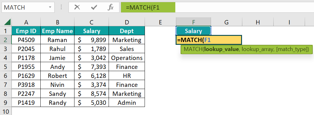
Select the lookup_value as cell F1.

Choose the lookup_array from A1:D1 because, in this range, we will find the column position of the lookup_value column “Salary”.

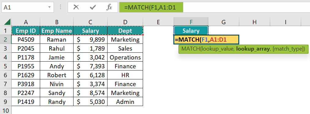
Next, choose the matching type as “Exact” by entering zero for the last argument.

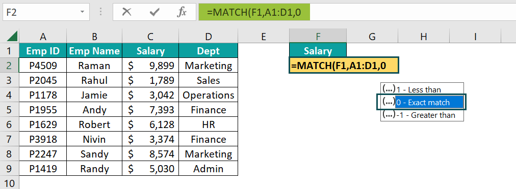
Close the brackets, and press the “Enter” key to get the column number for the header “Salary”.

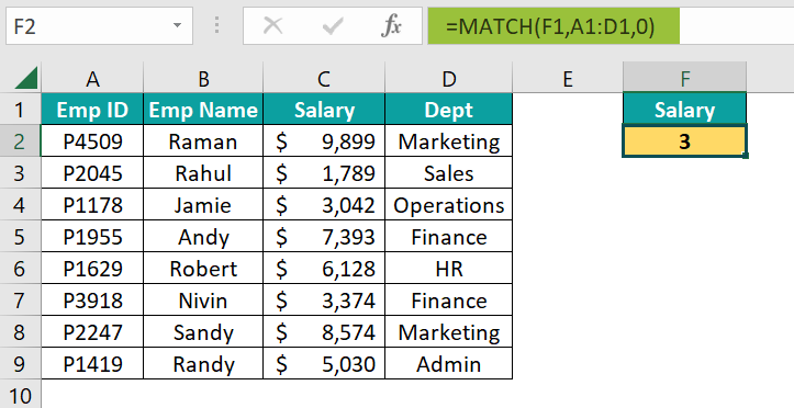
So, the column position of the header “Salary” in the range A1:D1 is 3, as shown above.

Let’s combine the VLOOKUP with the MATCH function to get the column index number dynamically.

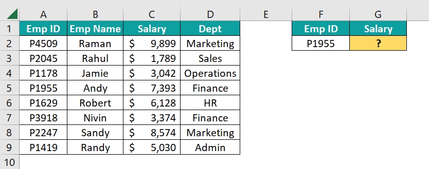
VLOOKUP with MATCH - Basic Example - VLOOKUP

The steps to find the salary information for employee id P1955 using VLOOKUP with MATCH are,

Enter the VLOOKUP function in cell G2.
Choose the lookup_value as cell F2.
Choose the table array from A2:D9.
Now, to specify the column index number, enter the MATCH function within the VLOOKUP function.
For the MATCH function lookup_value, choose the cell G1.
Choose the lookup_array from A1:D1.
Enter the matching type as 0 to get the exact match, and close the brackets.
For the last argument of the VLOOKUP function, enter the range lookup as FALSE or 0 for an exact match.
Close the brackets, and press the “Enter” key to get the result.

So, the salary information for the employee id “P1955” is $7,393.
The advantage of this method, i.e., VLOOKUP with MATCH, is that even when we delete or add new columns to the table array, we still get the correct result.

For instance, let us delete the “Employee Name” column from the table.

We are still getting the same salary information, unlike in the previous example. It is because the MATCH function returns the column number for the column header “Salary”. Before deleting the “Employee Name” column, the MATCH function gives 3 as the column number, and after deleting the “Employee Name” column, the function gives 2 as the column number.

So, the MATCH function dynamically returns the column index number for the VLOOKUP, and then the VLOOKUP function retrieves the value from the corresponding column.

Examples

We will consider some advanced scenarios using the VLOOKUP with MATCH.

Example #1 – VLOOKUP and the MATCH Function

We can allow the user to choose the desired result. For instance, look at the following data in Excel.

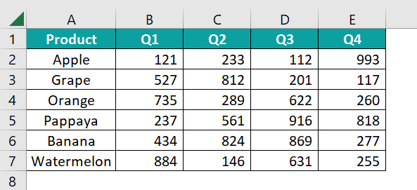
The steps to retrieve the result for the selected product and selected quarter are,

Step 1: Create a drop-down list of product items in cell G2.

Step 2: Similarly, create a drop-down list of quarters in cell H1 referencing cells B1:E1.

Step 3: Enter the VLOOKUP function in cell H2.

Step 4: Enter the lookup_value as product drop-down cell G2.

Step 5: Choose the table array from A2:E7.

Step 6: To get the column index number dynamically, enter the MATCH function inside the VLOOKUP function.

Step 7: Choose the lookup_value as a quarter drop-down cell H1.

Step 8: Choose the lookup_array from A1:E1.

Step 9: Enter the matching type as zero for the exact match and close the bracket.

Step 10: Next, for the range lookup argument of the VLOOKUP function, enter either FALSE or 0 for the exact match.

Close the brackets, and press the “Enter” key to get the following result.

As of now, we are getting an error an #N/A error.

Now, choose any of the products in cell G2, and any of the quarters in cell H1.

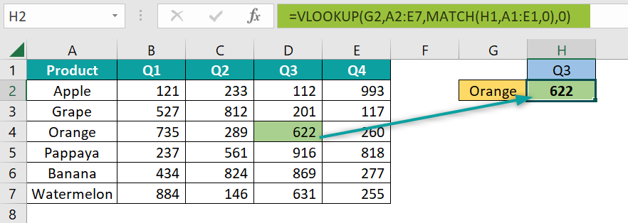
The units sold for the product “Orange” and the quarter “Q3” is 622. With this method, users can use the drop-down to select any combination of product and quarter, and retrieve the value for the same.

Example #2 – Use the MATCH Function to Avoid Manual Column Number Entry

If you are retrieving a greater number of columns, then providing the column index number of every one of those columns is time-consuming.

For instance, look at the following data in Excel.

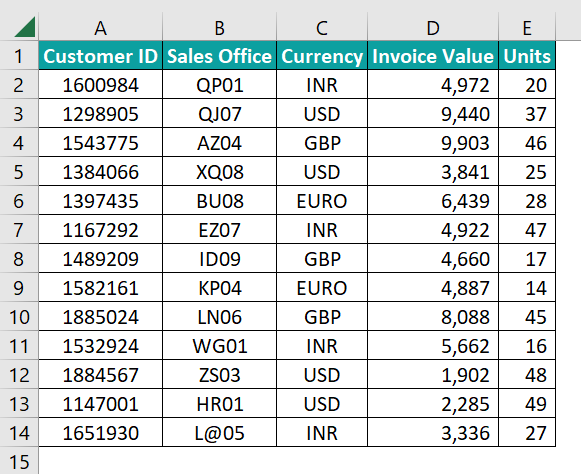
From this data, we are trying to retrieve the following information.

If we have to apply the VLOOKUP function with a static column index number, we need to apply it 3 times because, for every column, we need to mention the separate column index number.

Column numbers are also not in order, and for every column, we need to count the column index number and then mention those. Instead, apply the MATCH function to get the column index number dynamically.

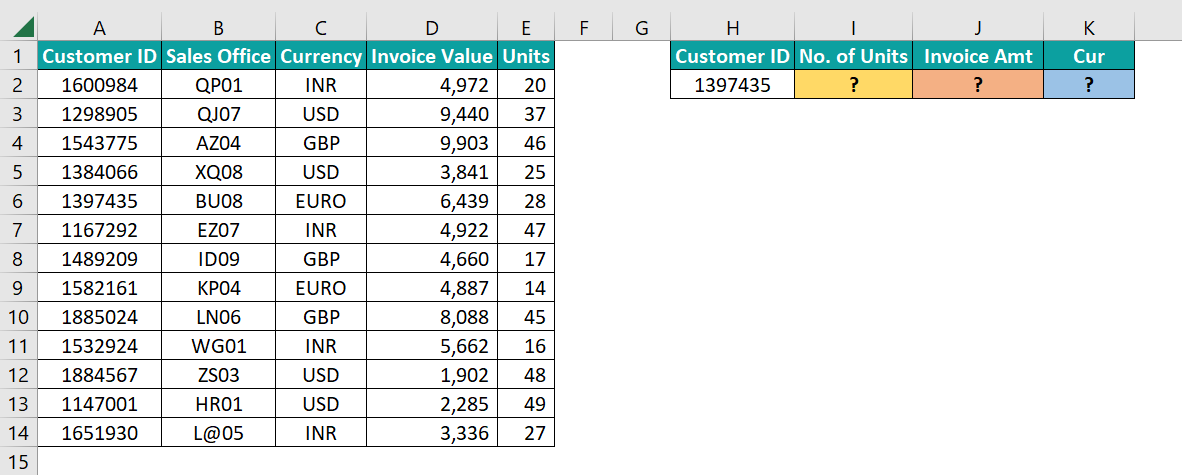
The steps to apply the MATCH function to get the column index number dynamically are,

Step 1: Enter the VLOOKUP function in cell I2.

Step 2: Enter the lookup_value as cell H2.

Step 3: Once the lookup_value cell reference is given, we need to make the column of this cell reference absolute by pressing the F4 key thrice. Because we will copy this formula to the right-side columns, the lookup_value should be the same.

[Note: The dollar sign ($) should come before the column header H.]

Step 4: Next, choose the table array from A2:E14 and make it an absolute reference by pressing the F4 key only once. Because once we copy the formula to other cells, this reference should be the same.

[Note: The dollar sign ($) should appear on either side of the column header and row header.]

Step 5: Next, to enter the column index number, we will enter the MATCH function.

Step 6: Choose the lookup_value as cell I1 and make the row reference by pressing the F4 key twice.

Step 7: Next, choose the lookup_array from A1:E1, and make this reference an absolute reference by pressing the F4 key once.

Step 8: Choose the matching type as 0 for the MATCH function and 0 for the VLOOKUP’s range lookup criteria. Because in both formulas, we are looking for the exact match.

Step 9: Close the brackets, and press the “Enter” key to get the following result.

We have got the result as an error (#N/A). There is a possible reason that the customer ID that we are looking for is not present in the table array range A2:E14. Let us check this first.

However, this customer id is available in the given table array.

Another possible reason is when we use the MATCH function, the column headers may not be the same in both instances.

In the table array, the column name is “Units”, but in the target table, the column name is “No. of Units”. So, the MATCH function did not find the exact match, hence returning no column numbers for the VLOOKUP function.

Hence, to make sure that the MATCH function works properly, the header should be the same in both instances.

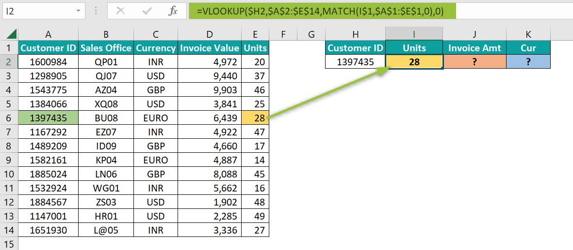
When we fixed the column header, we get the units sold for the customer id “1397435”.

Similarly, there is an issue with the other column headers as well.

Instead of “Invoice Value”, we have “Invoice Amt”, and instead of “Currency”, we have “Cur” in the target table. Correct these two column headers to get accurate results.

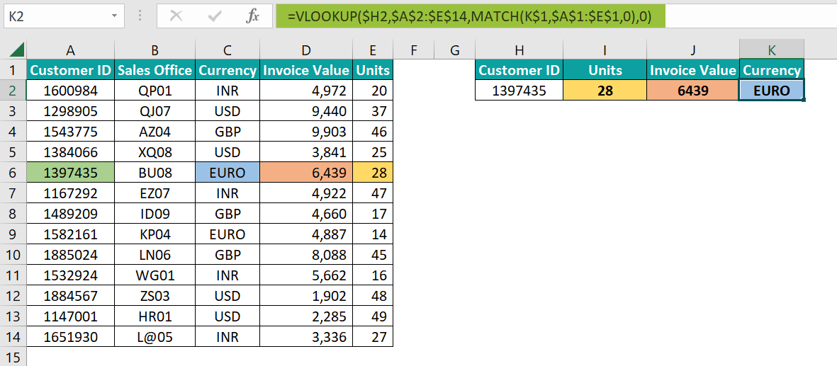
The accurate output is “EURO”, as shown above.

Important Things To Note

The VLOOKUP function does not consider the addition or deletion of the columns, so it will keep returning the result from the mentioned column index number.
When the MATCH function is used, we need not worry about the addition or deletion of the columns in the table array.
The MATCH function requires the lookup_value to be the same header name as in the table array.
Always make the table array reference absolute by pressing the F4 key once.
If any of the VLOOKUP and MATCH functions’ lookup_values does not match in the table array, we will get the #N/A error.

Frequently Asked Questions (FAQs)

1. How can VLOOKUP with MATCH help users?

When working on large datasets using the VLOOKUP function to retrieve certain column values, we may delete a few columns from the table. Then, a static column number will return a different column result than the desired one.
However, if we use the MATCH function to retrieve the column index number for the desired result column, then no need to worry about the addition or deletion of columns.

2. Why is VLOOKUP with MATCH Not Working?

The MATCH function will work if the header is the same in the table and the lookup_value cell. Even the slightest change, such as space, spelling error, etc., in the column header will result in a #N/A error.

3. What are the Limitations of VLOOKUP with MATCH?

• VLOOKUP and MATCH functions require the exact matching value in the lookup range. Even a space character will not consider it as a different value.
• If we opt for the approximate match, we are not sure whether it will return the correct result or not.
• To apply VLOOKUP with MATCH, the data should be vertically structured, and all the resulting columns should be to the right of the lookup_value column.

4. How to use VLOOKUP with MATCH and INDEX?

MATCH and INDEX functions are an alternative to the VLOOKUP function in Excel because VLOOKUP only fetches only from left to right of the lookup_value column.

For instance, look at the following data in Excel.

In cell E2, we are trying to fetch the “Sales Office” value for the customer id “1651930”. However, we cannot apply the VLOOKUP function here because the result column “Sales Office” is to the left of the lookup_value column “Customer ID”, so the VLOOKUP function doesn’t work.

To overcome this limitation, we can apply the INDEX and MATCH functions, as shown in the following image.

Therefore, the “Sales Office” for the customer id “1651930” is “L@05”.

Download Template

This article must help understand VLOOKUP with MATCH with its formulas and examples. You can download the template here to use it instantly.

VLOOKUP With MATCH Download

VLOOKUP With MATCH