
What is 3D Reference in Excel?
A 3D Reference in Excel refers to the same cell range or cells in different worksheets. It is one of the most remarkable features in Excel for cell references. It helps us conveniently perform calculations across several sheets containing the same data type.
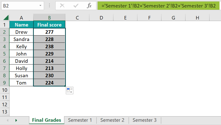
For example, let us consider some students’ marks in different worksheets for different semesters. To add each student’s scores across the different worksheets, type an = in cell B2 of the “Final Grades” worksheet. Go to each worksheet and select the corresponding cell B2 in each of them. You get the formula =‘Semester 1’!B2+’Semester 2’!B2+’Semester 3’!B2.
Use this 3D Reference in Excel Template to follow along with the examples in this article.
Download Excel TemplatePress Enter, and you get Drew’s score across three semesters. Then, drag the Autofill handle up to B9 to get the students’ final scores. Thus, you can use the 3D reference feature to perform calculations across worksheets that contain the same structure and data type.
Explanation
- As seen above, the 3D reference feature helps reference several worksheets containing the same data type and the same pattern, making calculations easy. In the above example, we try adding references from three sheets for a single analysis as they contain the same information/data type.
- In the formula, =‘Semester 1’!B2+’Semester 2’!B2+’Semester 3’!B2, each worksheet’s name is mentioned in single quotes (‘) after selection, and the “!” signifies the worksheet.
- Following the ‘!’ sign, you can add the cell reference/range required for the calculations.
- Rather than adding each worksheet name separately, you can specify consecutive worksheets and modify the formula as a 3D reference in the following way:
=SUM(Semester 1:Semester 3!B2)
Semester 1 and Semester 3 are the first and last worksheets, respectively. Therefore, we can use it when the worksheets have the same structure and are consecutively placed.
Key Takeaways
- A 3D reference in Excel refers to the same cell or range of cells on multiple worksheets, which can be used for long calculations. It is a critical feature in Excel that simplifies many complex calculations involving numerous worksheets.
- The functions that use 3D Reference in Excel include SUM, COUNT, VAR, PRODUCT, AVERAGE, MAX, MIN, etc.
- For a 3D reference in Excel, all the cell ranges/cells across the multiple worksheets should be of the same structure and data type.
How To Use 3-D Reference in Excel?
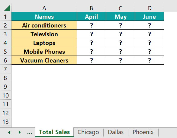
We can create a 3D Reference in Excel to find the total sales made on a company’s products over the months of April, May, and June in different cities. But first, we must calculate the total sales made in a worksheet called “Total Sales.”
Steps to use 3D references in excel are given below –
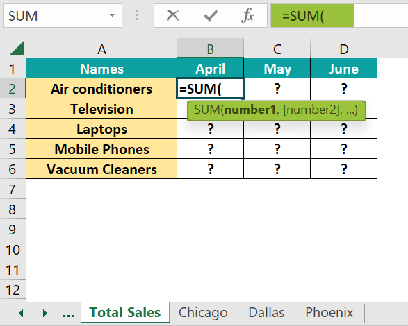
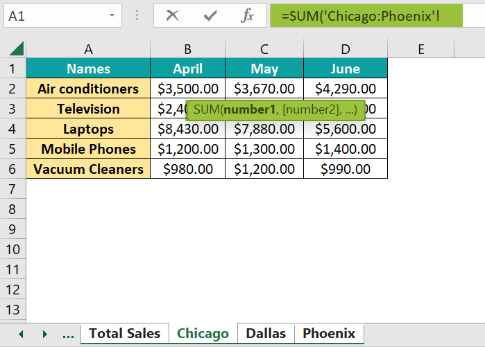
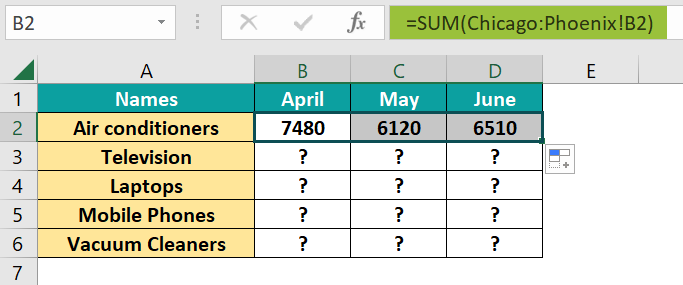
- Let us calculate the corresponding values in Columns B, C, and D for the three sheets for April, May, and June, respectively. In the “Total Sales” sheet, click on cell B2 and begin the formula as =SUM(.

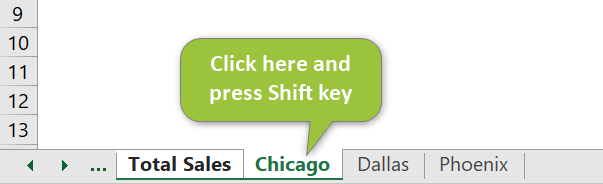
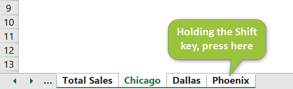
- Now, click on the worksheet named “Chicago” and press the Shift key.

- Next, click on the last worksheet to be included, that is, “Phoenix,” still holding the Shift key.
You get the formula modified like the one below.
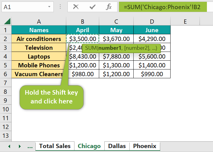
- Now, holding the Shift key down, click on the cell you want to calculate, B2, in this case.

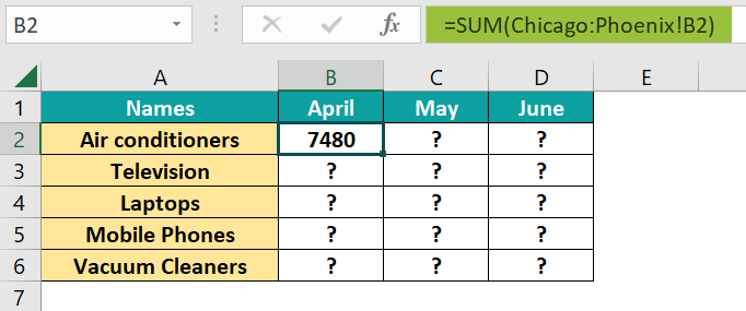
- Notice the change in the formula above. Now, release the Shift key, and press Enter. The total sales made in April for air conditioners across the three cities.

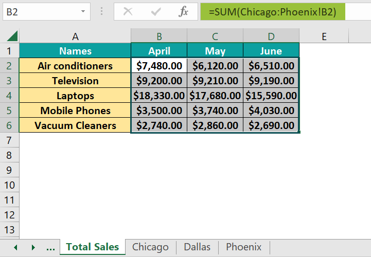
Drag the Autofill handle horizontally to get the air conditioners’ sales for all three months in all three cities.
- Drag it vertically to find the sales for other gadgets. We have applied Currency formatting to this range.

Thus, applying 3D reference in Excel is quick and saves time and effort.
Examples
Now that we have seen how to use the 3D Reference in Excel let us look at a few examples on this topic.
Example #1
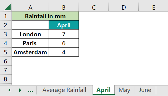
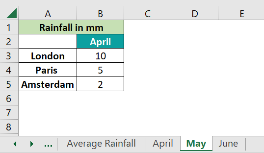
In this example, we have the rainfall received by three cities in April, May, and June. Let us calculate the average rainfall in these three cities over this period and plot a graph for better understanding.
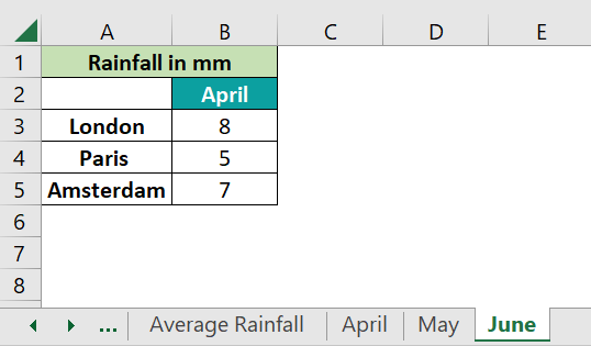
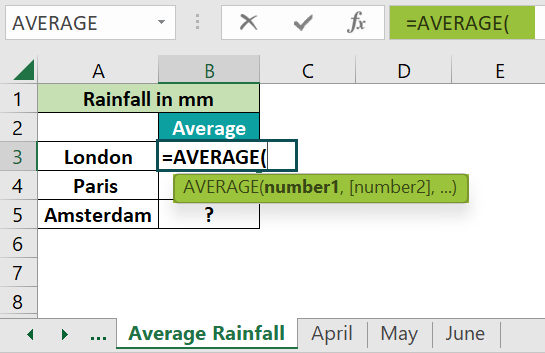
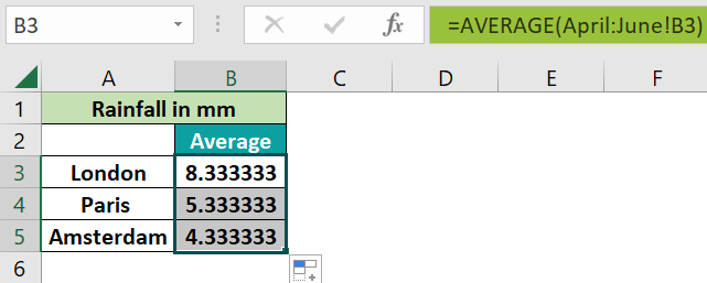
- Step 1: To find the average rainfall received in April, May, and June in the three cities, we have another worksheet called Average Rainfall for the 3D reference in Excel. Here, go to cell B3 and enter the following.
=AVERAGE(
- Step 2: Next, click on the tab “April.” Then, hold down the Shift key and click on “June.”
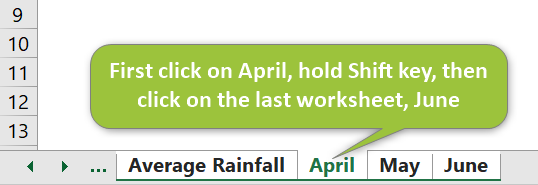
Now, click on cell B3. Press Enter after releasing the Shift key. You get the average rainfall in London for 3 months.
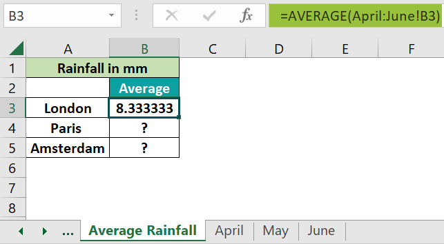
- Step 3: Drag the handle up to B5 to get the cities’ average.
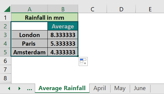
- Step 4: Select the required values in the Average Rainfall worksheet to plot a graph.
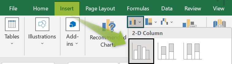
- Step 5: Go to the Insert tab, and click on the option “Insert Column or Bar Chart” in the Charts group.
Select the option Clustered Column charts in excel.
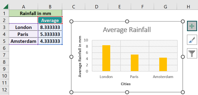
- Step 6: Now, we get the chart for the average rainfall. Click on the + sign on the top right side of the chart to add suitable labels.
Example #2
Let us take an example of a Café’s sheet. We include the annual details per quarter. Let us look at what happens if we must add a worksheet.
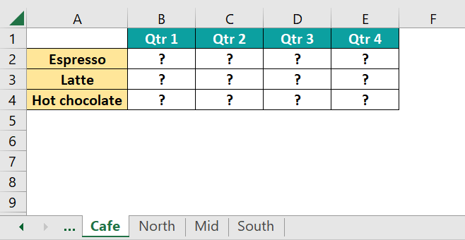
We must find the total sum for the details of the North, Mid, and South branches of the café.

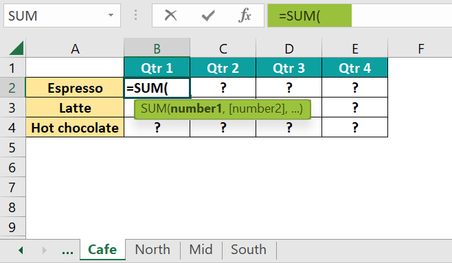
- Step 1: Go to the “Café” worksheet. Go to cell B2 and enter the following part of the formula.
=SUM(
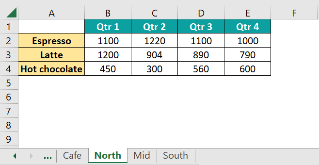
- Now, click on “North” in the worksheet tab.

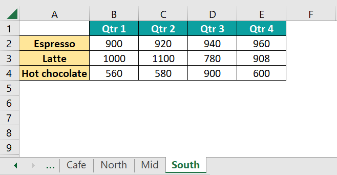
- Next, holding the “Shift” key down, click on the last worksheet, South.
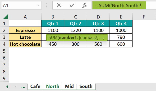
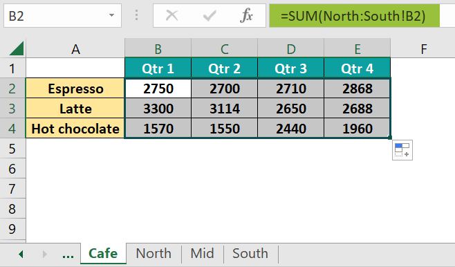
- Holding the Shift key, click on the cell/range of cells, B2 in this case, and press Enter. You get the total “Espresso” sales details for Qtr 1 in the worksheet Café.

- Step 2: Drag the Autofill handle horizontally and vertically, from B2 to E2 and B2 to B4, to get the sum for the first row and column. Repeat till all the columns are filled.
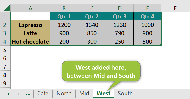
- Step 3: After all these calculations are done, you obtain the datasheet for the cafe in the West, which is to be integrated with the other sheets. Let us suppose you add this worksheet between Mid and South, as shown below.
- Step 4: Let us check if the formula and values in the Café worksheet are altered in any way.

The values in the main sheet Café are altered after we added the worksheet named West. However, since we added it between the first and last worksheet specified in the formula, the values are just integrated and added to the main sheet.
Example #3
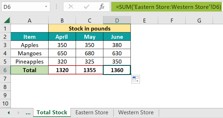
Let us look at another example where we prevent the cells from getting auto-formatted. Below are the stock details of some items in a store’s Eastern and Western branches for the months of April, May, and June. We must add the total stock quantity to know the main store details using the SUM excel function and 3D Reference in Excel.
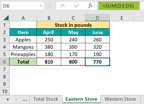
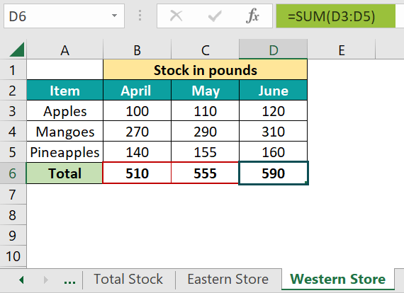
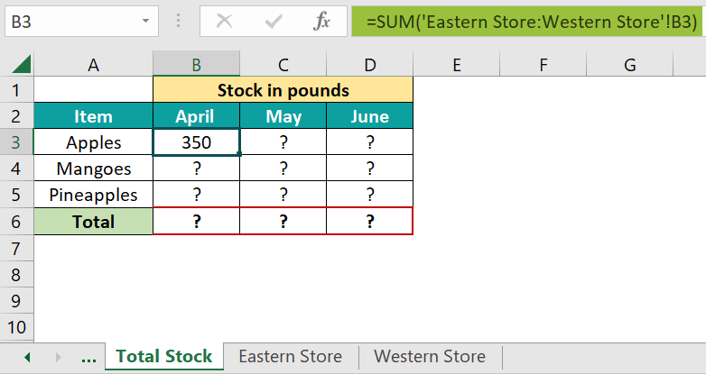
- Step 1: Notice the formatting of the cells. To get the total stocks, we begin to insert 3D Reference in Excel by typing the following formula in cell B3 of the Total Stock worksheet: =SUM(
- Next, click on the sheet “Eastern Store”, hold down the Shift key and click on the “Western Store” tab.
- Select the cell that you want to add, B3, in this case, and press Enter.
You get the total stock of apples for May.
- Step 2: Drag the Autofill handle from B2 to D5 and B2 to B5.
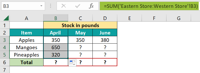
- Step 3: When you try to drag the handle from B5 to B6, you can notice a change in the formatting of the boundary. It is because the red boundary changes to a normal black one since the formatting has also been copied from the previous cell.
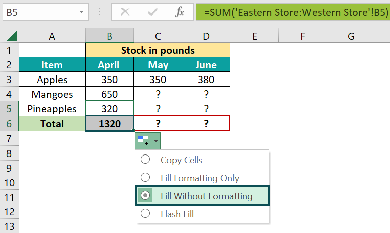
To avoid this, click on the small box in the right corner called “Autofill excel options.”

- Step 4: Choose the “Fill without Formatting” option.
- Step 5: Repeat the same for cells C6 and D6 as well. You will notice that the formatting is not changed. Thus, you can apply the formula to different cells without choosing the formatting.
Important Points to Note
- If you insert a worksheet between the first and last worksheet specified in the 3D reference formula, then Excel includes all its values in the calculations.
- Similarly, if you delete a worksheet that is present in the specified formula range, Excel removes those values from the calculation.
- If the first or last worksheet specified in the formula is removed, its values are also removed from the calculation, and the endpoint is shifted to the previous worksheet. If the first worksheet is deleted, the next becomes the starting point.
- The formula does not display all the worksheets but only the first and last worksheets separated by a ‘:’.
- Hold the Shift key down to select the last worksheet for your formula and the cell/cell range to be included in the calculations.
Frequently Asked Questions (FAQs)
For the 3D reference in Excel, we also can define names. In the Formulas tab, select Define Name in the Defined Names group. In the New Name dialog box that pops up, enter the details like Name and the range.
If the worksheets are not placed one after the other, and we use the 3D reference formula, it does not work. Also, the cell ranges selected for calculation should have the same structure across the sheets. Besides, the sequence of the worksheets should be as specified in the formula.
The formula is as follows:
=SUM(First_worksheet:Last_worksheet!cell/cell range)
It is a convenient way to calculate the same cells in more than one sheet. While using complex formulas across different sheets might be tedious, with the Excel 3-D formula, you must specify the sheets to be included, eliminating a lot of hard work.
Use this 3D Reference in Excel Template to follow along with the examples in this article.
Download Excel Template