
What Is ADDRESS In Google Sheets?
ADDRESS in Google sheets, as the name suggests, helps users find the cell address in the form of a text. It is a default function available in both Excel and Google sheets. ADDRESS function in Google sheets is used for data analysis and project management. It is a straight forward function used to manage the spreadsheet cells.
For example, let us learn how to find the cell address of a value with the row number and column number 8 and 10, respectively. Now, let us learn how to find the result using ADDRESS function in Google sheets.
Use this ADDRESS In Google Sheets Template to follow along with the examples in this article.
Download Excel TemplateTo begin with, we need to enter the ADDRESS function in Google sheets formula, =ADDRESS(8,10) in cell A1.

Press Enter key. We will be able to see the result in cell A1, as shown in the below image.

Likewise, we will be able to see the result in Google sheets. In this article, let us learn how to use the ADDRESS function in Google sheets with detailed examples.
Key Takeaways
- ADDRESS function in Google sheets, in simple terms is the function specifying the cell address of a value.
- The formula of ADDRESS function in Google sheets is =ADDRESS(row,column,[absolute_relative_mode],[use_a1_notation],[sheet]) where row and column are the mandatory arguments showing the row number and column number, respectively.
- The optional arguments, absolute_relative_mode, use_A1_notation and sheet are the optional arguments used in the formula.
- Remember, the use_a1_notation can be represented in two formats – A1 and R1C1, where, TRUE is the default value and the result is obtained in the A1 notation. If we use R1C1 notation, we need to use FALSE as the value.
Syntax

The formula or syntax of ADDRESS function in Google sheets is =ADDRESS(row,column,[absolute_relative_mode],[use_a1_notation],[sheet])
where,
- row is the mandatory argument showing the row number
- column is the mandatory argument showing the column number
- absolute_relative_mode is the optional arguments showing values 1, 2, 3, and 4. Let us learn the meaning of these values.
- use_a1_notation can be represented in two formats – TRUE and FALSE. These values are based on the formats used in the formula. The formats are mostly in A1 format. The second format is R1C1.
- A1 represents the column in letters followed by the rows in numbers.
- R1C1 represents the row number followed by the column number.
- TRUE is the default value and the result is obtained in the A1 notation. If we use R1C1 notation, we need to use FALSE as the value.
- sheet is the optional argument showing the name of the sheets where we want to specify the cell.
How To Use ADDRESS In Google Sheets?
We can use the ADDRESS in Google sheets with two different methods. They are:
- Select the ADDRESS function under the Insert tab
- Manually enter the ADDRESS function
Method #1 – Select the ADDRESS function under the Insert tab
The steps to select the ADDRESS function under the Insert tab are:
Step 1: To begin with, we need to enter the data in the spreadsheet. Next, we need to select the cell where we want to find the result.
Step 2: Now, we need to select the Insert tab and click on the Functions option. In the list of function category, we need to click on the Lookup function category and then, click on the ADDRESS function in Google sheets.

Step 3: We will be able to see the formula in Google sheets. Now, click on the necessary arguments.
Step 4: Press Enter key. We will be able to see the result in the active cell.
Likewise, we can use the ADDRESS function in Google sheets using the Insert tab.
Method #2 – Manually enter the ADDRESS function
The steps to manually select the ADDRESS function are:
Step 1: To begin with, we need to enter the data in the spreadsheet. Next, we need to select the cell where we want to find the result.
Step 2: Now, we need to enter =AD in the cell. Select the ADDRESS function formula in Google sheets.

Step 3: Alternatively, we can also direct =ADDRESS directly in Google sheets.
Step 4: We will be able to see the formula. Now, click on the necessary arguments.
Step 5: Press Enter key. We will be able to see the result in the active cell.
Likewise, we can use the ADDRESS function in Google sheets manually.
Examples
Now, let us learn how to use the ADDRESS function in Google sheets with the help of the below examples.
Example #1 – Combine ADDRESS And INDIRECT
For example, consider the below table showing name and marks in columns A and B, respectively.

Now, let us learn how to find the result using ADDRESS and INDIRECT function in Google sheets.
The steps to find the result are:
Step 1: To begin with, we need to enter the data in the spreadsheet. In this example, the data is available in the cell range A1:B8. Next, we need to select the cell where we want to find the result. In this example, we need to select the cell E2.
Step 2: Now, enter the ADDRESS function in cell E2.
So, the complete formula is =ADDRESS(2,2).

Step 3: Press Enter key. We will be able to see the result in the cell E2.

Step 4: Now, let us find the data associated with the cell address using the INDIRECT function in Google sheets formula.
So, enter the INDIRECT function formula, =INDIRECT(E2) in cell E3.

Step 5: Press Enter key. We will be able to see the result as shown in the below image.

Likewise, we can use the ADDRESS function in Google sheets with the INDIRECT function.
Example #2 – Combine ADDRESS And MATCH
For better understanding, let us use the same example we used in example 1.
Consider the below table showing name and marks in columns A and B, respectively.

Now, let us learn how to find the result using ADDRESS and MATCH function in Google sheets.
The steps to find the result are:
Step 1: To begin with, we need to enter the data in the spreadsheet. In this example, the data is available in the cell range A1:B8. Next, we need to select the cell where we want to find the result. In this example, we need to select the cell E2.
Step 2: Now, enter the MAX function in cell E2.
So, the complete formula is =MAX(B2:B8).

Step 3: Press Enter key. We will be able to see the result in the cell E2.

Step 4: Now, let us find the data associated with the cell address using the ADDRESS and MATCH function in Google sheets formula.
So, enter the ADDRESS function formula with MATCH function, =ADDRESS(Match(E2,$B:$B,0),2) in cell E3.

Step 5: Press Enter key. We will be able to see the result as shown in the below image.

Likewise, we can use the ADDRESS function in Google sheets with the MATCH function.
Example #3 – Combine ADDRESS And SUBSTITUTE
For example, consider the below table showing semester and marks in columns A and B, respectively.

Now, let us learn how to find the result using ADDRESS and SUBSTITUTE function in Google sheets.
The steps to find the result are:
Step 1: To begin with, we need to enter the data in the spreadsheet. In this example, the data is available in the cell range A1:B8. Next, we need to select the cell where we want to find the result. In this example, we need to select the cell D2.
Step 2: Now, enter the ADDRESS and SUBSTITUTE function in cell D2.
So, the complete formula is =SUBSTITUTE(ADDRESS(1,A2,4),”1″,””).

Step 3: Press Enter key. We will be able to see the result in the cell E2.

Likewise, we can use the ADDRESS function in Google sheets with the SUBSTITUTE function.
Example #4 – Find The Cell With The Highest Or Lowest Value
For example, consider the below table showing subject and marks in columns A and B, respectively.

Now, let us learn how to find the cell with the highest or the lowest value using ADDRESS function in Google sheets.
The steps to find the cell with the lowest value are:
Step 1: To begin with, we need to enter the data in the spreadsheet. In this example, the data is available in the cell range A1:B8. Next, we need to select the cell where we want to find the result. In this example, we need to select the cell E2.
Step 2: Now, enter the MIN function in cell E2.
So, the complete formula is =MIN(B2:B8)

Step 3: Press Enter key. We will be able to see the result in the cell E2.

Step 4: Now, let us find the data associated with the cell address using the ADDRESS function in Google sheets formula with a combination of MATCH and MIN functions.
So, enter the function formula, =ADDRESS(Match(Min(B2:B8),B1:B8,0),Column(B1)) in cell E3.

Step 5: Press Enter key. We will be able to see the result as shown in the below image.

Likewise, we can use the ADDRESS function in Google sheets to find the highest or lowest call value.
Important Things To Note
- ADDRESS function in Google sheets is a default function used to find the cell address of a value in the spreadsheet.
- It is highly used to organize, identify the cell containing the data.
- Remember, we need to make sure to enter the required values in the argument to avoid errors like #VALUE! Error.
Frequently Asked Questions (FAQs)
For example, let us learn how to find the cell address of a value with the row number and column number 5 and 5, respectively.
Now, let us learn how to find the result using ADDRESS function in Google sheets.
To begin with, we need to enter the ADDRESS function in Google sheets formula, =ADDRESS(5,5) in cell A1.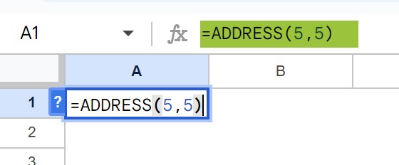
Press Enter key. We will be able to see the result in cell A1, as shown in the below image.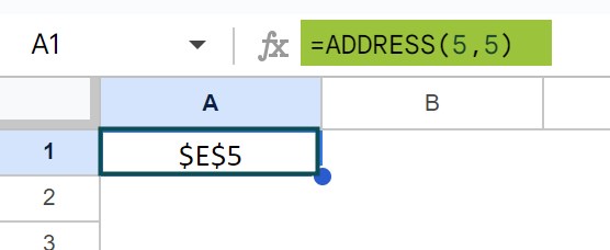
Likewise, we will be able to see the result in Google sheets.
ADDRESS function in Google sheets may not work properly if:
• The syntax is not properly mentioned in the argument and formula
•If the data does not match with the formula used.
We need to use the MAX function in Google sheets to find the maximum value. Then, we need to use the combination of ADDRESS function with the MATCH and MAX function in Google sheets.
Use this ADDRESS In Google Sheets Template to follow along with the examples in this article.
Download Excel TemplateRecommended Articles
Continue with these related resources when you want the next practical step in this topic.
- Basic Google Sheets Formulas
- Google Sheets Functions
- Array Formula In Google Sheets
- Comparison Operators in Google Sheets
- Relative References in Google Sheets
Explore the full Google Sheets Formula Basics guide or browse Google Sheets Resources.