CHAR Function In Google Sheets

What Is CHAR Function In Google Sheets?

The CHAR function in Google Sheets helps users convert a value that is a number, alphabet or arithmetic symbols, into a special symbol according to the chosen ASCII code or UNICODE table. It is also the inverse of the Google Sheets CODE, which returns the ASCII codes for the specified characters.

Users can utilize the Google Sheets CHAR function when translating code page numbers, writing mathematical or chemical formulas, inserting a line break into the given text value, etc. For example, we will write the following formula in a right manner using the Google Sheets CHAR function.

CHAR-Function-In-Google-Sheets-Deinition

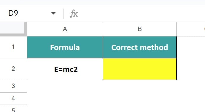
Select cell B2, enter the formula =“E=mc”&Char(178) and press “Enter”.

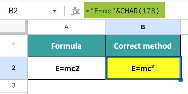
CHAR-Function-In-Google-Sheets-Deinition-1

The output is shown above. The value 2 is raised to the power or to the superscript position using the CHAR function.

The CHAR function in Google Sheets determines the character specified by the given number.
We can use the function to,
- Write the chemical or mathematical formulas in the precise format.
- Insert subscript or superscript, which is a drawback in Google Sheets as this feature is not available.
- Combine address or any other values using Ampersand (&), add Line Breaks, hyphen, or any special symbols.
- Convert page numbers in files received from other computer systems into characters
The CHAR() accepts one argument, number, as input, which can be any code from the 1 to 255 range of the ASCII code or the millions of code of the UNICODE.
Since CHAR is the inverse of the CODE function, if we are unable to get the ASCII code for a character, then we can use the CODE function to get the CHAR number. However, we must ensure to enter the character as a cell reference or a cell value within double-quotes.

Syntax

The syntax of the CHAR Google Sheets formula is,

The one and only mandatory argument of the CHAR formula in Google Sheets is,

table_number: It is a number specifying the character we require from the character set defined in our computer’s operating system. The value of this argument can range between 1 and 255.

How To Use CHAR Function In Google Sheets?

We can use the CHAR Function in Google Sheets in two ways, as follows:

Access from the Google Sheets ribbon.
Enter the formula in the worksheet manually.

Method #1 – Access from the Goggle Sheets ribbon

Step 1: Choose an empty cell for the output – select the “Insert” tab – click the “Function” option right arrow – click the “Text” option right arrow – select the “CHAR” function, as shown below.

Step 2: The “CHAR” formula appears, as shown below. Enter the argument as cell value or cell reference and press “Enter”.

Method #2 – Enter the formula in the worksheet manually

Step 1: Select an empty cell for the output.

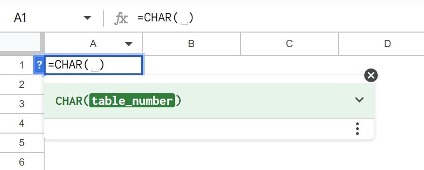
Step 2: Type =CHAR( in the cell, as shown below. [Alternatively, type =C or =CH and double-click the CHAR from the Google Sheets suggestions.]

Step 3: Enter the argument as cell value or cell reference.

Step 4: Close the brackets and press “Enter”.

Examples

To understand it effectively, let us see some more CHAR function in Google Sheets examples.

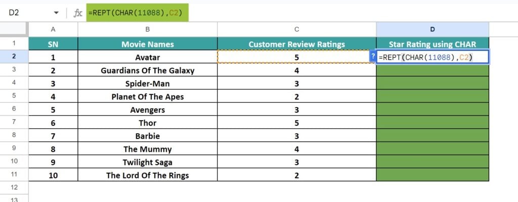
Exampple #1 – Star Rating for cutomer reviews

The dataset given below consists of Top 10 movies that has sequels and their ratings. We will use the

CHAR function to insert Star Rating for customer reviews

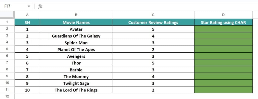
CHAR-Function-In-Google-Sheets-Example-1

The steps to insert the symbol STAR for the ratings using the CHAR() are as follows:

Step 1: Select cell D2 and enter the formula =REPT(CHAR(11088),C2), as shown below.

[Note: REPT function repeats the selected text for the specified number of times.]

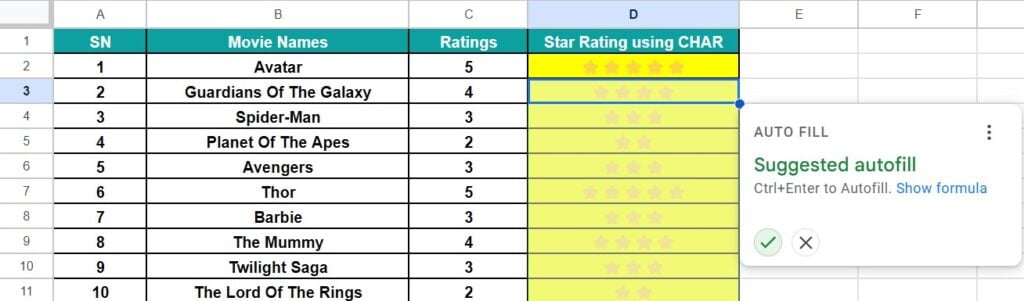
Step 2: Press “Enter” and immediately the Google Sheets provides the autofill suggestion, as shown below, either choose it or use the fill handle method.

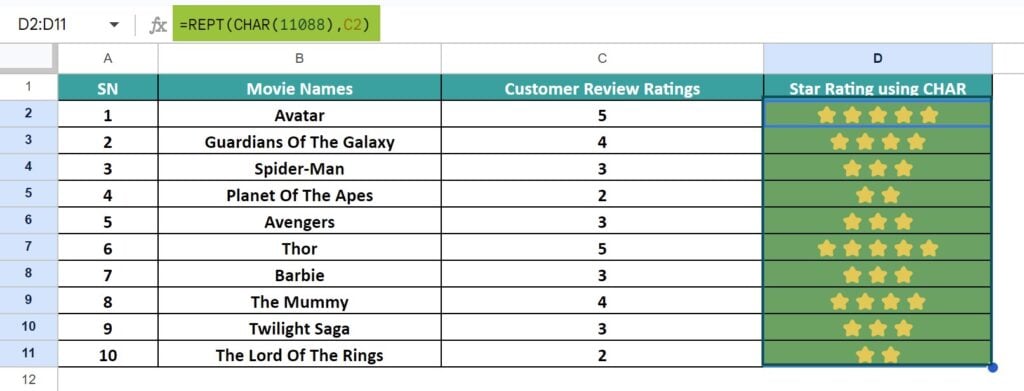
Step 3: Drag the formula from cell D2 to D11 using the fill handle to get the following results.

Example #2 – Upward-Downward Pointing Arrows

In the dataset given below we have the arrow positions mentioned. We will convert it into symbols using the CHAR function.

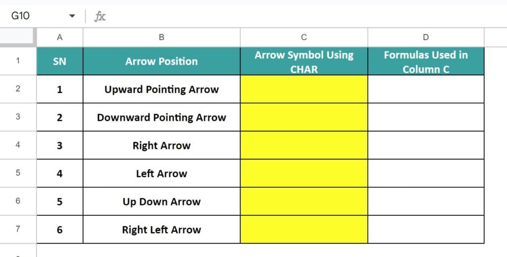
CHAR-Function-In-Google-Sheets-Example-2

The steps to convert the Upward-Downward Pointing Arrows and some other arrow positions to symbol using the CHAR function are as follows:

Select cell C2, enter the formula =CHAR(8593) and press “Enter”.
Select cell C3, enter the formula =CHAR(8595) and press “Enter”.
Select cell C4, enter the formula =CHAR(8594) and press “Enter”.
Select cell C5, enter the formula =CHAR(8592) and press “Enter”.
Select cell C6, enter the formula =CHAR(8597) and press “Enter”.
Select cell C7, enter the formula =CHAR(8596) and press “Enter”.

CHAR-Function-In-Google-Sheets-Example-2-1

The convert to symbol output is shown above in column C and in Column D we have entered the formulas used in the corresponding Column C cells, for our reference.

Example #3 – Symbol Combined with Text

We will combine the text vales given in the dataset with a linking symbol using the Ampersand (&) and the CHAR function.

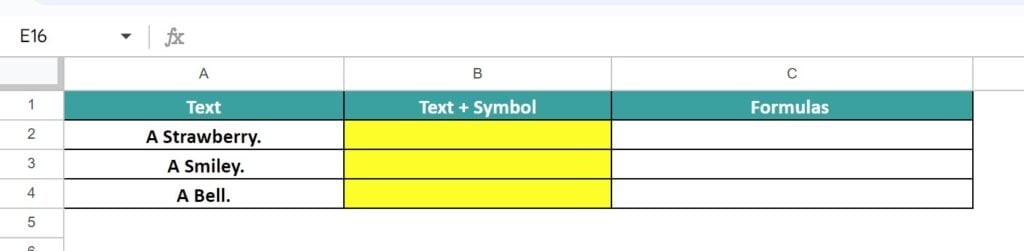
CHAR-Function-In-Google-Sheets-Example-3

The steps to insert Symbol Combined with Text using the CHAR function are as follows:

Select cell B2, enter the formula =A2&CHAR(127827) and press “Enter”.
Select cell B3, enter the formula =A3&CHAR(128512) and press “Enter”.
Select cell B4, enter the formula =A4&CHAR(128276) and press “Enter”.

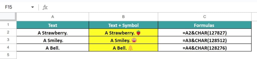
CHAR-Function-In-Google-Sheets-Example-3-1

The output is shown above. Column C is for our reference.

Example #4 -Superscript and Subscript

Consider the dataset given below of some chemical and mathematical formulas. We will rewrite them in the correct form using the CHAR function to convert some characters to Superscript and Subscript and also use the Ampersand (&).

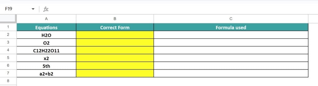
CHAR-Function-In-Google-Sheets-Example-4

The steps to convert a few letters to Superscript and Subscript using the CHAR function are as follows:

Select cell B2, enter the formula =”H”&CHAR(8322)&”O” and press “Enter”.
Select cell B3, enter the formula =”O”&CHAR(8322) and press “Enter”.
Select cell B4, enter the formula =”C”&CHAR(8321)&CHAR(8322)&”H”&CHAR(8322)&CHAR(8322)&”O”&CHAR(8321)&CHAR(8321) and press “Enter”.
Select cell B5, enter the formula =”x”&CHAR(178) and press “Enter”.
Select cell B6, enter the formula =”5″&CHAR(7511)&CHAR(688) and press “Enter”.
Select cell B7, enter the formula =”a”&CHAR(178)&”+b”&CHAR(178) and press “Enter”.

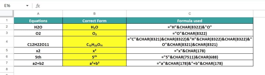
CHAR-Function-In-Google-Sheets-Example-4-1

The output is shown above. Again, column C is for our reference to understand the formulas used in column B.

Important Things To Note

The CHAR function in Google Sheets returns a string or text value.
We can enter the CHAR() argument directly as the cell value or cell reference.
If the argument number is not between 1 and 255, then we will get the #NUM! error.

Frequently Asked Questions (FAQs)

1. Why is the CHAR in Google Sheets not working?

The CHAR in Google Sheets might not work due to the following reasons;
a. The UNICODE provided is invalid.
b. If Ampersand (&) is used to combine the cell values and are not provided within double-quotes, unless it is a cell reference, then we will get an incorrect output.
c. The argument values entered is non-numeric or does not fall within the range of 1 to 255.

2. What is an alternate way to insert the CHAR in Google Sheets?

We often forget in which category a function falls, here, the “CHAR” function. Then, we can insert the function as follows:
Choose an empty cell -select the “Insert” tab -click the “Function” option right arrow – click the “All” option right arrow – select the “CHAR” function, as shown below.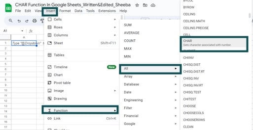
FAQ-2
However, as always, entering the function manually is the best way to avoid confusion.

3. Where else can we find the CHAR in Google Sheets?

Alternatively, we can find the Functions icon to insert the CHAR in Google Sheets by following the path shown below.
Choose an empty cell – click the “More” option represented by the three vertical dots at the end of the toolbar, as shown below.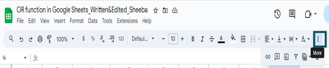
FAQ-3
A list of icons appears when we click the “More” option. Here, click the “Functions” icon, as shown below.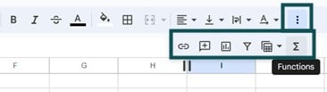
FAQ-3-1
Here, click the “Functions” option – click the “All” option right arrow – select the “CHAR” function, as shown below.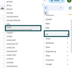
FAQ-3-2

4. How can we find a CHAR number for the CHAR function in Google Sheets?

We already know that CHAR function is the inverse of the CODE function in Google Sheets, which returns the code for a specified character. Therefore, we can find a CHAR number using the CODE().
For example, the table below contains a list of characters. We will find the Char numbers using the CODE function and then cross verify the results.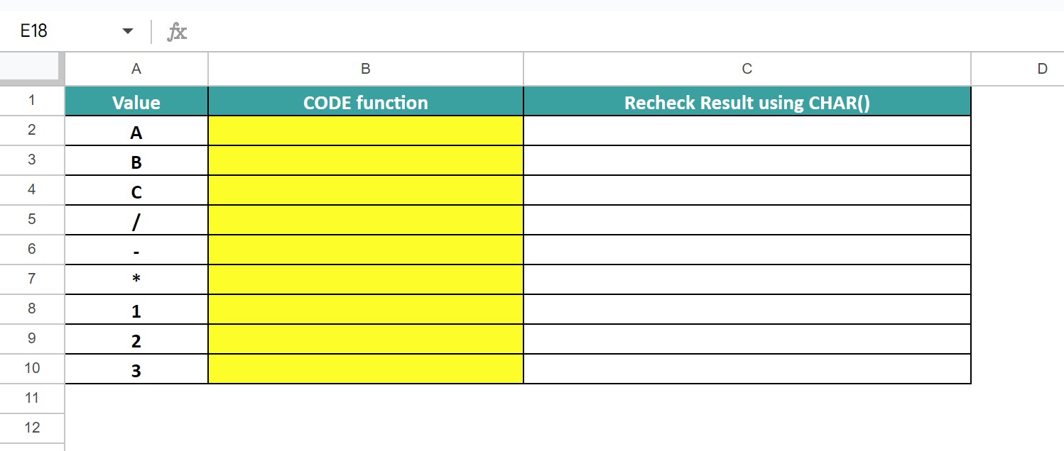
FAQ-4
First, select cell B2, enter the formula =CODE(A2), press “Enter” and once we get the output, drag the formula from cell B2 to B10 using the fill handle.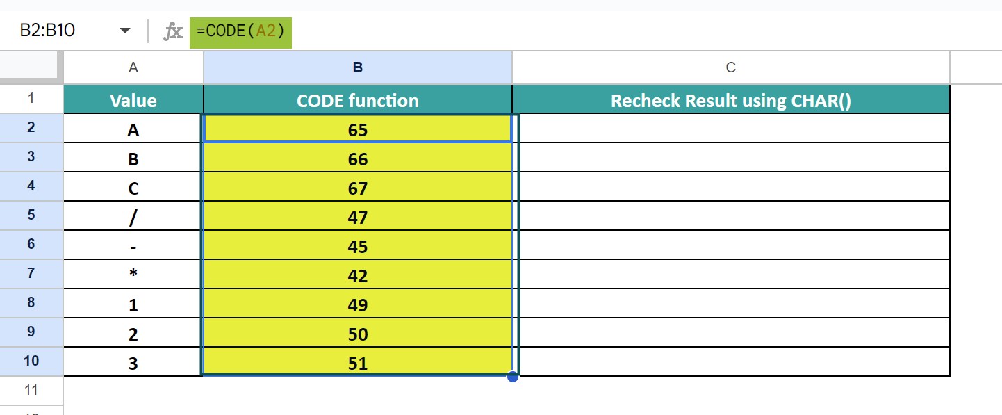

FAQ-4-1
Now, select cell C2, enter the formula =CHAR(B2), press “Enter” and once we get the output, drag the formula from cell C2 to C10 using the fill handle.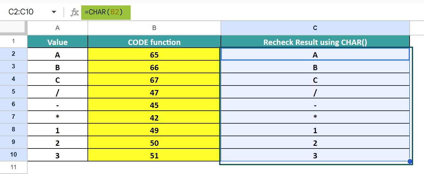

FAQ-4-2
The output is shown above. We see that the CODE function retrieved the ASCII code of the letters. As we verified the CHAR function returned the same letters with the generated code. This proves that the CODE function is the inverse of the Char function.

Download Template

This article must be helpful to understand the CHAR Function in Google Sheets, with its formula and examples. You can download the template here to use it instantly.

CHAR-Function-In-Google-Sheets Download

CHAR Function In Google Sheets