What Is Excel Column Merge?
Column merge in Excel is an option to combine two or more columns of data into one column. And while one can merge columns within a worksheet, merging columns across multiple worksheets and files is feasible.
Users can merge columns in Excel to organize and format data spread across multiple columns into one column, which helps sort data and remove duplicate entries.
For example, the table below contains ten students’ first and last names.

And the requirement is to display each student’s full name using their first and last names in column F. Then, we can perform two column merge in Excel by using the CONCAT() or the ‘&’ symbol in the target cells to obtain the required outcome.

In the above two column merge in Excel example, the CONCAT() accepts three inputs, a student’s first name, a space character, and the student’s last name.
Alternatively, we can use the ‘&’ symbol-based two column merge in Excel formula to combine each student’s first name, a space character, and the last name.
Both methods merge the two columns, D and E, data in each row with a space character in between to display each student’s full name in column F.
Table of contents
Key Takeaways
- Column merge in Excel is a method that helps concatenate the data in multiple columns across one or more sheets and files and display the combined data in one column.
- Users can merge columns in a spreadsheet to logically organize massive datasets in fewer columns.
- We can use the CONCAT() and the ‘&’ operator to merge columns in Excel.
- We can supply cell values and references as inputs to the column merge formulas. And we can manipulate column values and merge them with texts, constants, and special characters according to our data concatenation requirements.
How To Merge Multiple Columns In Excel?
We can combine multiple columns in Excel by using the following methods:
- Using the CONCAT Function
- Merge the Cells by Using the “&” Symbol
Method #1 – Using The CONCAT Function
The CONCAT() combines specified values from multiple ranges without delimiters.
And the steps to perform column merge in Excel by applying the CONCAT() are as follows:
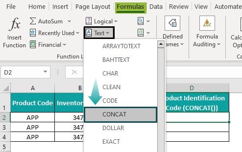
- Choose a target cell and select the Formulas tab – the Text drop-down – select the CONCAT function.

- The Function Arguments window will open.
Here, we must update the mandatory Text1 field, followed by the required number of optional fields Text2, Text3, and so on, as values or Excel cell references to values.
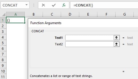
Please note that the CONCAT() can accept up to 255 arguments as input. And if the resulting concatenated value contains more than 32767 characters, the function output will be the #VALUE! error in Excel.
- Click OK in the Function Arguments window to view the CONCAT() output in the target cell.
Alternatively, we can directly enter the CONCAT() in the target cell using the following steps:
- Choose a target cell to display the output.
- Enter =CONCAT( in the target cell. [ Alternatively, enter =C or =CON and double-click the CONCAT function from the Excel suggestions.]
- Supply the arguments as cell values or references to the values and close the brackets.
- Press Enter to execute the function and view the required column merge in Excel output.
Ensure the supplied arguments are without any syntax errors in both methods. Otherwise, we may face a scenario of the column merge in Excel not working.
Example #1
The table below lists product codes, inventory codes, and products.

And the requirement is to create a product identification code in each row of column D by merging columns A: C data using the CONCAT(). Then, the steps are as follows:
Step 1: Choose the target cell D2 and select the Formulas tab – Text – CONCAT function.
Step 2: Enter the argument values, as shown below.
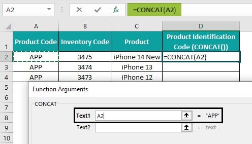
And once we click on the second argument field, the third argument field will appear.

So, we can update as many argument fields according to the requirement, as depicted below.
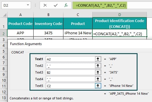
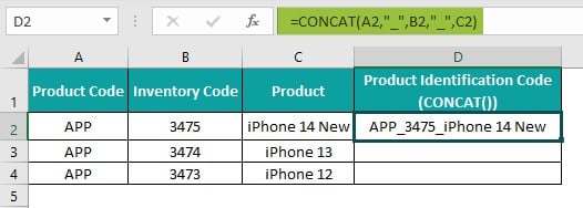
Step 3: Click OK in the Function Arguments window to view the CONCAT() output in the target cell D2.
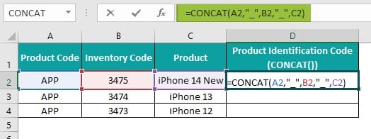
[ Alternatively, select cell D2 and type the CONCAT().
=CONCAT(A2,”_”,B2,”_”,C2)
And pressing Enter will result in the required output.]
The CONCAT() accepts the cell references to the columns A:C cells, with underscores in double quotes in between. And it merges the three columns’ cells to return the output as APP_3475_iPhone 14 New.
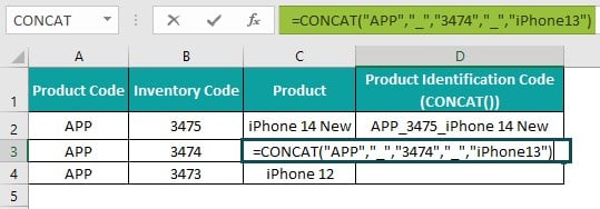
Step 4: Select cell D3 and enter the CONCAT().
=CONCAT(“APP”,”_”,3474,”_”,”iPhone 13″)
Step 5: Press Enter to view the CONCAT() return value.
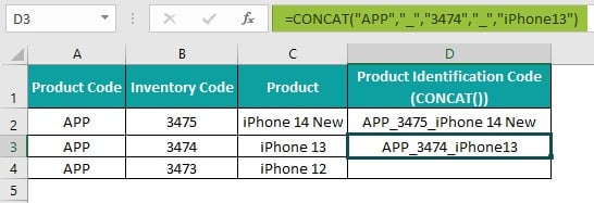
The CONCAT() accepts the values in the columns A:C cells, A3:C3, with text values within double quotes and the number value without double quotes. And it combines the cells in the three columns to return the output, APP_3474_iPhone 13.
Step 6: Choose cell D4 and enter the CONCAT().
=CONCAT(A4:B4&”_”,C4)
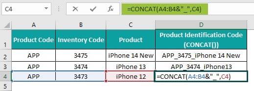
Next, select the first argument in the CONCAT(), A4:B4&”_”, and press F9 to convert the cell range reference to values.
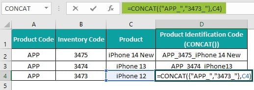
Next, press Enter to view the outcome, as shown below.
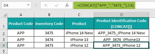
When we select the first argument, A4:B4&”_” inside the CONCAT() and press F9, it shows the cells A4 and B4 values with appended underscore symbols as an array. And then, when we press Enter to execute the resulting formula, it combines the array values and the third column cell C4 value to return the value APP_3473_iPhone 12.
The above formula will be useful when we need to include the same symbol between a range of column values.
Method #2 – Merge The Cells By Using The “&” Symbol
The steps to perform column merge in Excel by using the ‘&’ symbol are as follows:
- Choose a target cell to display the output.
- Enter the ‘=’ symbol, the first column cell value or reference to the value, the ‘&’ symbol. And then, enter the remaining columns’ cell values or cell references to the values and required characters, with the ‘&’ symbol between each value.
- Press Enter to view the column merge in Excel formula output.
Example #2
The table below contains the username, domain name and extension details.

And the requirement is to generate an e-mail address based on the given data and display the outcome in cell D2.
Then, here is how to use the ‘&’ symbol to merge the given data in cells A2:C2 in columns A, B, and C and achieve the desired output in the target cell D2.
Step 1: Select cell D2 and enter the following formula.
=A2&”@”&B2&”.”&C2

Step 2: Press Enter to view the formula output, allen1990@gmail.com

Likewise, we can directly enter the values specified in cells A2:C2 to merge the corresponding columns of data using the ‘&’ symbol.
And as the given cell values and special characters are texts, we must provide them in double quotes. Otherwise, we will face the condition of column merge in Excel not working.
=”allen1990″&”@”&”gmail”&”.”&”com”

The ‘&’ symbol concatenates the specified values. And thus, the output appears as the required columns merged.
Example #3
The table below lists the top best sellers and their author details.

And the requirement is to merge the columns A and B data and display the output in column C in the column C title format. Then, we can use the CONCAT() in the target cells and obtain the required output.
Step 1: Choose the target cell C2, enter the CONCAT(), and press Enter.
=CONCAT(A2,”: “,B2)

Step 2: Update the formula in cells C3:C6 using the Excel fill handle.

The CONCAT() in each row accepts three inputs, the corresponding column A cell value, ‘: ‘, and column B cell value. And it concatenates the three specified values to return an output that shows the two columns, A and B, merged.
We can also use the ‘&’ symbol to create a two column merge in Excel formula in the target cells and achieve the same output as above.
And for that, choose cell C2, enter the following formula, and press Enter.
=A2&”: “&B2

And then utilize the fill handle to enter the formula in the remaining target cells.

The ‘&’ symbol combines the three input values in the specified order to result in an output that shows the two columns, A and B, merged into one column, C.
Example #4
We shall see the steps to merge columns in different sheets.
Consider we have two worksheets in a workbook, Values and Arithmetic Operators. While the first sheet contains two sets of values, the second lists arithmetic operators.
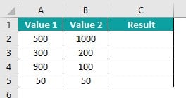
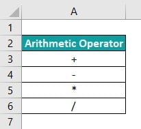
And we must merge columns A and B values of the Values sheet with column A data in the Arithmetic Operators worksheet to show and perform the specified arithmetic operations. And assume the target cells are in column C of the Values sheet.
Then, we can use the CONCAT() in the target cells to show the output as the merged column values.
Step 1: Select cell C2, enter the CONCAT() as shown below:
=CONCAT(A2,” “,

Next, go to the second sheet and click cell A3 to select the required arithmetic operator.
=CONCAT(A2,” “,’Arithmetic Operators’!A3

And then, add a comma, click the Values sheet tab, and select cell B2 to choose the second value.
=CONCAT(A2,” “,’Arithmetic Operators’!A3,” “,Values!B2

And then, enter a comma, ‘ = ‘, with a space character before and after it, and the last argument as the formula to perform the corresponding arithmetic operation.
=CONCAT(A2,” “,’Arithmetic Operators’!A3,” “,Values!B2,” = “,(A2+B2))

Finally, press Enter to execute the function.

Likewise, we can update the formulas in the remaining target cells.
Step 2: Choose cell C3, enter the CONCAT(), and press Enter.
=CONCAT(A3,” “,’Arithmetic Operators’!A4,” “,Values!B3,” = “,(A3-B3))

Step 3: Choose cell C4, enter the CONCAT(), and press Enter.
=CONCAT(A4,” “,’Arithmetic Operators’!A5,” “,Values!B4,” = “,(A4*B4))

Step 4: Choose cell C5, enter the CONCAT(), and press Enter.
=CONCAT(A5,” “,’Arithmetic Operators’!A6,” “,Values!B5,” = “,(A5/B5))

The CONCAT() in each row accepts seven inputs. And since we refer to the column A value from the Arithmetic Operators sheet in the Values sheet, the second sheet name appears before the corresponding cell reference. And as we return to the Values sheet to refer to column B cell, the first sheet name appears before the cell reference, after which we can complete the formula as usual.
First, the last argument in the CONCAT() executes to return the specified arithmetic operation output. And then, the CONCAT() concatenates the inputs to return the output as the merged column values.
Example #5
The table below lists the top US stocks and their price change percentages.

And the requirement is to show the given data as a comment in each row of column C. Then, we can use the ‘&’ symbol to merge columns A and B values to show the required comments.
Step 1: Select cell C2, enter the following formula, and press Enter.
=”The price change percentage in the Stock “&A2&” is: “&TEXT(B2,”0.00%”)&”.”

Step 2: Use the fill handle to enter the formula in the remaining target cells.

First, the TEXT Excel function displays the price change value as a percentage, according to the specified number format. And then, the ‘&’ symbol merges the given texts and the two columns, A and B, values in the specified order to return the required comment in each target cell.
Please note that when we use the CONCAT() or the ‘&’ symbol to merge columns, the output shows numeric values in the number format interpreted by Excel. For example, a percentage will appear in the decimal format, and a date value will display as a serial number.
Thus, using functions like TEXT to display values in the desired format is important.
Important Things To Note
- The formulas to column merge in Excel are case-sensitive. So, ensure to provide the column text values in the appropriate cases for merging.
- Consider we need to merge columns with cells containing numbers such as percentages, dates, and time values. Then, use the TEXT() in the column merge formula to display the numbers in the required formats in the output.
- The CONCAT() is available from Excel 2016 onwards. So, if the Excel version is older than 2016, use the CONCATENATE Excel function to merge columns.
- The CONCAT() can accept up to 255 argument values. And if its return value contains over 32767 characters, the CONCAT() output is the #VALUE! error.

Frequently Asked Question (FAQs)
We can merge 4 columns in Excel by applying the CONCAT().
For example, the table below shows an employee’s name, birth month, and the date and month of joining the company.
And the requirement is to create an employee ID using the first two letters of the employee name and birth month, joining date, and the first two letters of the joining month. Assume the target cell is E2.
Then, we can use the CONCAT() with LEFT() in the target cell to obtain the required output.
Step 1: Choose cell E2, enter the CONCAT(), and press Enter.
=CONCAT(LEFT(A2,2),LEFT(B2,2),C2,LEFT(D2,2))
First, the three instances of the LEFT() return the first two letters of the cells A2, B2, and D2 values, JO, JA, and AP. Next, the CONCAT() combines the manipulated columns A, B, and D values and column C value in the order A to D to merge them. And it returns the required employee ID, JOJA5AP, in the target cell.
We can merge a date and time column in Excel utilizing the ‘&’ symbol with the TEXT().
For example, the table below shows a report ID and its generation date and time.
And the requirement is to update the report generation details as a statement in cell D2. Then, we can merge columns A, B, and C values using the ‘&’ symbol.
Step 1: Select cell D2, enter the following formula, and press Enter.
=”Report “&A2&” Generation Date & Time: “&TEXT(B2,”DD-MMM-YYYY”)&” “&TEXT(C2,”HH:MM:SS”)
First, the two TEXT() instances display the date and time values according to the specified date and time formats. Otherwise, the date and time will appear as a serial number and decimal in the output.
And then, the ‘&’ symbol merges the specified texts and the column values to return the required output in the target cell.
You can merge two columns in Excel using Flash Fill in the following way, which we will see with an example.
The table below shows two columns, A and B, listing the Microsoft applications and their official colors.
And the requirement is to merge columns A and B data using Flash Fill and display the concatenated data in column C.
Step 1: Choose cell C2, enter or copy the cell A2 value, enter ‘:’, enter or copy the cell B2 value, and press Enter.
Step 2: Select cell C2 or the cell below it. And then, select the Data tab – Flash Fill function or use the keys Ctrl + E to access the Flash Fill feature.
The Flash Fill feature will immediately update the remaining target cells using the same filling pattern we applied to populate cell C2.
However, this method will not work if we use the column merge formulas to update cell C2.
Download Template
This article must be helpful to understand the Column Merge In Excel, with its formula and examples. You can download the template here to use it instantly.
Recommended Articles
This has been a guide to What Is Column Merge In Excel. We explain how to merge them using two different methods with examples and points to remember. You can learn more from the following articles –

Leave a Reply