
What Is CONVERT Function In Excel?
The CONVERT function in Excel helps users to convert a numeric value’s measuring unit to another, such as miles to kilometers, kilograms to grams, pounds to dollars, etc., or vice versa. The CONVERT Excel function is an inbuilt Engineering function, so we can insert the formula from the “Function Library” or enter it directly in the worksheet.
For example, the below table contains a list of numbers and their respective units in columns A and B.
Use this CONVERT Function In Excel Template to follow along with the examples in this article.
Download Excel Template
We will convert the above values using the CONVERT function. First, select cell E2, enter the formula =CONVERT(A2,B2,C2), press “Enter”, and drag the formula from cell E2 to E4 using the fill handle.
The output is shown above. The function accepts the given number, its unit, and the new unit to be converted to. Column F is for our reference.
Key Takeaways
- The CONVERT function in Excel converts the number specified in one measurement system to another measurement system within the same group.
- In the 3 mandatory arguments, number, from_unit, and to_unit, the first argument is a number, and the function accepts the second and third arguments as text values in double quotations.
- We can use the CONVERT() as a standalone function, or with other Excel functions such as VLOOKUP(), ROUND(), etc.
- The unit names and prefixes provided as arguments to the CONVERT() are case-sensitive.
CONVERT() Excel Formula
The syntax of the CONVERT Excel formula is:

The arguments of the CONVERT Excel formula are:
- number: The numeric value in the measurement unit we require to convert.
- from_unit: The unit we require to convert the given number from.
- to_unit: The unit we require to convert the given number to.
All the arguments in the CONVERT function in Excel are mandatory. While the first argument is a number, the function accepts the second and third arguments as text values in double quotations.
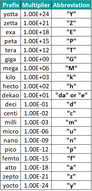
The following tables show the text values (units in different measurement systems under each group) that the CONVERT function in Excel accepts as the second and third arguments.


On the other hand, we can prep the abbreviated unit prefixes listed in the first table to any metric unit. And we can use the binary prefixes provided in the second table with “bits and “bytes”.

How To Use CONVERT Excel Function?
We can use the CONVERT function in Excel in 2 methods, namely,
- Access from the Excel ribbon
- Enter in the worksheet manually
Method #1 – Access from the Excel ribbon
First, choose an empty cell → select the “Formulas” tab → go to the “Function Library” → click the “More Functions” option drop-down → click the “Engineering” option right arrow → select the “CONVERT” function, as shown below.

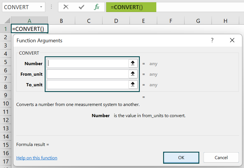
The “Function Arguments” window appears. Enter the argument values in the “Number”, “From_unit”, and “To_unit” fields → click “OK”, as shown below.
Method #2 – Enter in the worksheet manually
- Select an empty cell for the output.
- Type =CONVERT( in the cell. [Alternatively, type =C and select the CONVERT function from the Excel suggestions.
- Enter the arguments as cell values or cell references.
- Close the brackets and press Enter to view the converted number.
Let us take an example to understand this function.
We will convert the numbers to the required measuring units using CONVERT function in Excel.
Consider the following table containing a list of values and their respective units in columns A and B.

The steps to convert the values using CONVERT function in Excel are,
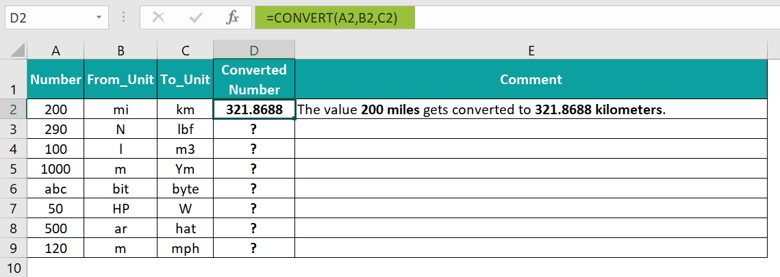
- First, select cell D2, enter the formula =CONVERT(A2,B2,C2), and press Enter.

[Alternatively, select cell D2 → click Formulas → More Functions → Engineering → CONVERT. This step will open the Function Arguments window.
Enter the three argument values in the Function Arguments window, as shown below.
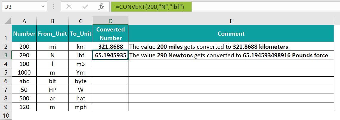
And once we click OK, the output, 321.8688, will appear in cell D2.] - Now, select cell D3, enter the formula =CONVERT(290,”N”,”lbf”), and press Enter.
[As the first argument is a number, we do not need to enter the value in double quotations. And as the unit arguments are text values, we must enter them in double quotes.]
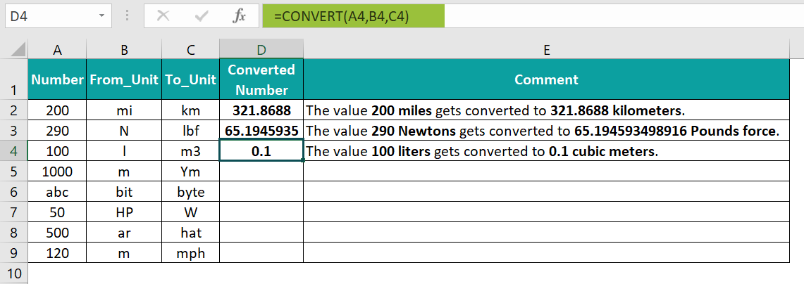
- Select cell D4, enter the formula =CONVERT(A4,B4,C4), and press Enter.
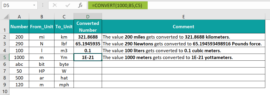
- Next, select cell D5, enter the formula =CONVERT(1000,B5,C5), and press Enter.
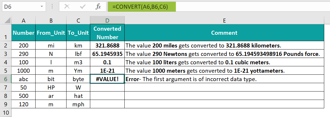
[Here, the requirement is to convert meters to yottameters. So the CONVERT() in the target cell D5 includes the metric prefix, yotta, prepended to the third argument, to_unit.] - Select cell D6, enter the formula =CONVERT(A6,B6,C6), and press Enter.
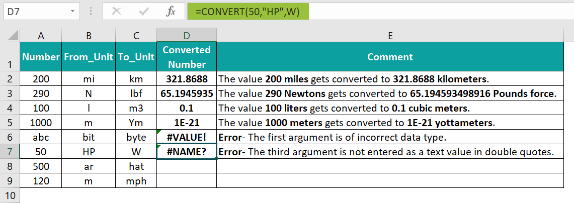
[As the argument number is a text instead of a numeric value, the CONVERT() output in the target cell D6 is the #VALUE! error.] - Then, select cell D7, enter the formula =CONVERT(50,”HP”,W), and press Enter.
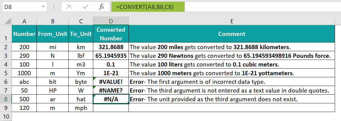
[The CONVERT() in the target cell D7 returns the #NAME? error since the third argument value, W, is not in double quotations.] - Select cell D8, enter the formula =CONVERT(A8,B8,C8), and press Enter.
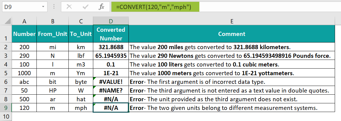
[The third argument value, hat, in row 8 does not exist in the Area measurement system or any other metric system. And thus, the function returns the #N/A error.] - Finally, select cell D9, enter the formula =CONVERT(120,”m”,”mph”), and press Enter.
[The CONVERT() in the target cell D9 returns the #N/A error, as the two specified units are from different groups, Distance, and Speed. And hence the conversion is not possible.]
The converted measuring units are shown above.


Examples
We will understand different scenarios with the CONVERT function in Excel examples.
Example #1
We will convert the land area data in square meters using the CONVERT function.
The below table contains a list of US states and their land area data in square miles.

The steps to convert the values using the CONVERT function in Excel are,
- Step 1: Select cell C2, enter the formula =CONVERT(B2,”mi2″,”m2″), and press Enter.

- Step 2: Drag the formula from cell C2 to C11 using the fill handle.

We get the output as shown above.
[Output Observation: Let us see the target cell C11 formula to understand how it works. The first argument, number, is the value 96003. And the second and third arguments are mi2 and m2, the units for square miles and square meters. And, as 1 square mile is equal to 2.59e+6 square meters, the CONVERT function in Excel returns 2.48647E+11 square meters as the output.
[Note: We may also enter the above formula in the following ways to achieve the same result,
=CONVERT(B11,”mi^2″,”m^2″)
Or
=CONVERT(CONVERT(B11,”mi”,”m”),”mi”,”m”) ]
Example #2
We will determine the speed of each car in meters/second using the CONVERT function.
The table below shows a list of cars and the distances they cover in the specified hours. Here, the given distance values are miles, and the time values are hours.

The steps to convert the values using the CONVERT function in Excel are,
- Step 1: Select cell D2, enter the formula =CONVERT(B2,”mi”,”m”)/CONVERT(C2,”hr”,”sec”), and press Enter.
[The CONVERT() in the numerator accepts the distance value, 38, and the units of miles and meters, mi and m, as inputs. And it converts the distance value, 38 miles, to 61155.072 meters.
On the other hand, the CONVERT() in the denominator takes the hour value, 2, and the units of hours and seconds, hr and sec, as inputs. It then converts the hour value, 2 hours, to 7200 seconds.
And finally, the division formula divides the two values to return 8.49376 meters/second.]

- Step 2: Drag the formula from cell D2 to D6 using the fill handle.

We get the output as shown above.
Example #3
We will use the CONVERT function in Excel with VLOOKUP(), and ROUND(), to determine the temperature of the country, Mauritania, and display the value in Degree Fahrenheit.
In the following image, the first table contains a list of the top 10 hottest countries in 2022, based on their average annual temperature in Degree Celsius.

The procedure to use the CONVERT function in Excel with ROUND() and VLOOKUP() is,
- Select cell F2, enter the formula =ROUND(CONVERT(VLOOKUP(E2,A:B,2,0),”C”,”F”),2), and press Enter.

The output is shown above.
Output Observation:
First, the VLOOKUP() looks up the country name, Mauritania, in the first table to return its temperature value in Degree Celsius, 28.34.
Then the CONVERT() accepts 28.34 as the firstargument and the units for Degree Celsius and Fahrenheit, C, and F, as the second and third arguments. And it returns the temperature value in Degree Fahrenheit, 83.012.
Finally, the ROUND() rounds the temperature value to two decimal places to return the output as 83.01.
Important Things to Note
- The CONVERT function in Excel returns the #VALUE! error when the supplied arguments have incorrect data types.
- We will get the #NAME? error when we supply the unit arguments directly without double quotations.
- The CONVERT() returns the #N/A error in three scenarios:
- If the supplied unit arguments do not exist.
- The specified unit does not support a binary prefix.
- And, if the provided units belong to different groups.
Frequently Asked Questions (FAQs)
The CONVERT function is in the Formulas tab. We must click Formulas → More Functions → Engineering → CONVERT to apply it in the required cell.
We can utilize the CONVERT() in Excel VBA using the method:
Application.WorksheetFunction.Convert(number,from_unit,to_unit)
For example, the below table contains a list of numbers and their respective units in columns A and B.
The steps to convert the given values using the CONVERT() in Excel and VBA are,
• 1: In the worksheet with the above table, press the keys Alt + F11 to open the VBA Editor.
• 2: Select the required VBAProject and select the option Insert → Module to open a new Module window, Module1.
• 3: Type the VBA code, as shown in the below image, in the Module1 window to apply the CONVERT() in the target cells.
Sub CONVERT_fn()
Range(“E2”) = Application.WorksheetFunction.Convert(Range(“A2”), Range(“B2”), Range(“C2”))
Range(“E3”) = Application.WorksheetFunction.Convert(Range(“A3”), Range(“B3”), Range(“C3”))
Range(“E4”) = Application.WorksheetFunction.Convert(Range(“A4”), Range(“B4”), Range(“C4”))
End Sub
• 4: Click the Run Sub/UserForm button in the top menu to execute the entered VBA code.
Once we execute the code, we will get the converted numbers in the corresponding target cells, as shown below.
We can convert inches to square feet by using the CONVERT function in Excel.
For example, the below table contains a list of values in inches.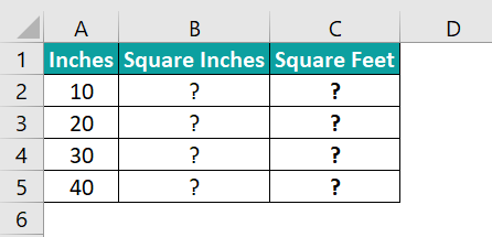
The steps to convert values using the CONVERT function in Excel are,
• 1: First, to convert inches to square feet, we will determine the corresponding square inches value for each given inch value. So, select cell B2, enter the formula =A2*A2, and press Enter.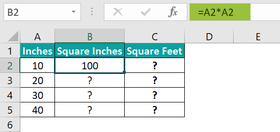
• 2: Drag the formula from cell B2 to B5 using the fill handle.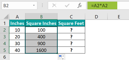
• 3: Next, to convert the square inches values to square feet values using the CONVERT(), select cell C2, enter the formula =CONVERT(B2,”in^2″,”ft^2″), and press Enter.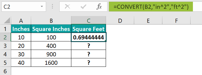
• 4: Drag the formula from cell C2 to C5 using the fill handle.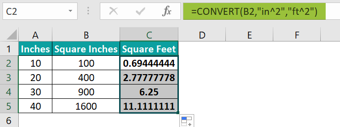
We get the output as shown above.
[Output Observation: The CONVERT() in each target cell takes the corresponding square inches value as the first argument. And the second and third arguments are in^2 and ft^2, the units for square inches and square feet.
Thus, the CONVERT() returns the respective square feet values in column C, based on the inputs.]
Use this CONVERT Function In Excel Template to follow along with the examples in this article.
Download Excel Template