COUNTIFS Function in Excel

What Is COUNTIFS Function In Excel?

COUNTIFS as the name suggests, it is the improved version of the COUNTIF function where it was designed to take only one criterion to count something.

The COUNTIFS function in Excel takes multiple criteria into consideration. To count something based on several criteria in Excel, the COUNTIFS function will be the go-to formula. The COUNTIFS function in excel is available from Excel 2007 onwards versions. For instance, look at the following data in Excel.

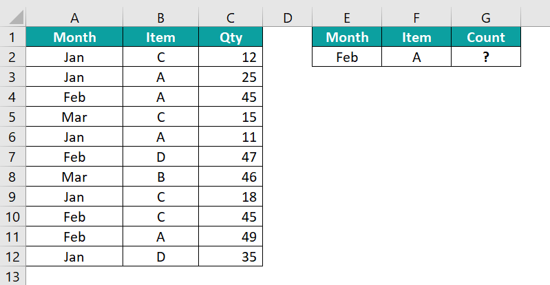
We have some data in the range A1:C12. In cell G2 we need to get the count of the item “A” for the month “Feb”. Next, enter the following formula in cell G2 to get the count.

=COUNTIFS(A2:A12,E2,B2:B12,F2)

As we can see, the count for item “A” in the month “Feb” is 2. In these two criteria combinations, we have 2 line items in the range A2:C12.

COUNTIFS() Excel Formula

The COUNTIFS function in excel formula is very much like the COUNTIF Excel function.

• Criteria Range 1: First we need to select the criteria range in which criteria 1 will be evaluated.

• Criteria 1: From Criteria Range 1 what cells are to be counted. We can supply the condition in the form of text (in the double quote), number, Excel cell reference, or any other excel function input.

• [Criteria Range 2]: This is an optional argument. Here we need to select the second criteria range in which [Criteria 2] will be evaluated.

• [Criteria 2]: This is also an optional argument. We can supply the second condition to be considered within the criteria range 2.

We can specify up to 127 criteria ranges and criteria in the COUNTIFS function. We need not have to remember any of the syntaxes because MS Excel will display the syntax after every argument.

How To Use COUNTIFS Excel Function?

Let us have a basic example of using COUNTIFS function in Excel. We will use the following data in Excel for this example.

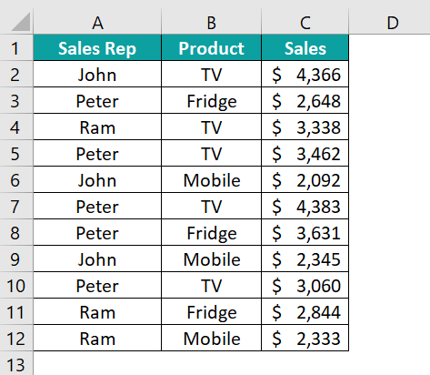
We have sales data based on sales representatives who sold multiple products. Now we need to know the sales rep “Peter” has sold how many TVs.

Examples

Example #1 – Two Conditions (Multiple Criteria)

Now let us move into some of the advanced examples of using COUNTIFS function in Excel. Going forward we will use the following data in Excel for all the examples.

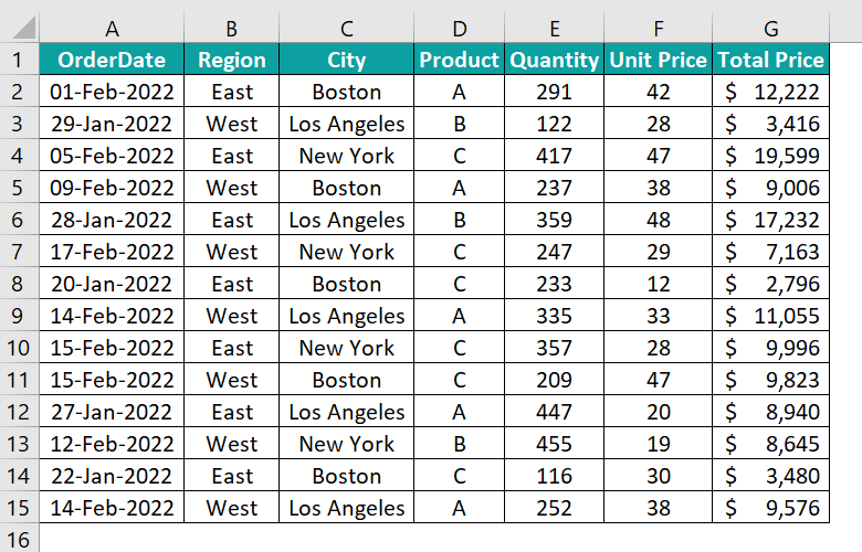
From the above sales data, we need to create a summary table like the following.

We need to find in each how many times each product has sold.

• Step 1: To begin with, enter the COUNTIFS function in cell J3.

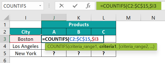
• Step 2: Next, choose the criteria range as the city column from C2:C15. After the selection, we need to make this reference an absolute reference because the same reference will be copied to the other cells as well.

After the range selection, press the F4 key once to make the selection an absolute reference.

Note: As we can see we have dollar symbols on either side of the row and column to suggest it as an absolute reference.

• Step 3: Then, choose the criteria as cell I3. This criteria reference should be mixed. Next, insert an absolute reference to the column by pressing the F4 key thrice.

• Step 4: Choose the second criterion as the product column from the range D2:D15. Make this reference an absolute by pressing the F4 key once.

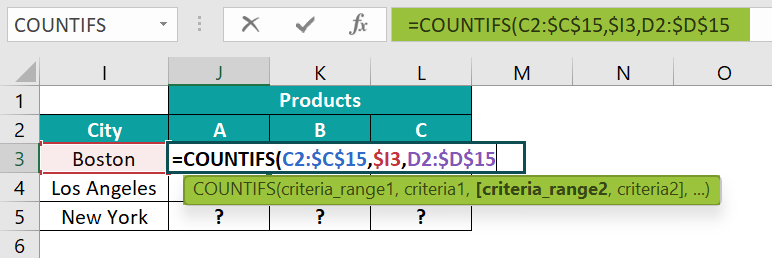
• Step 5: Choose criteria 2 as cell J2. Make this cell reference mixed by making the row an absolute reference by pressing F4 key twice.

• Step 6: Close the bracket and hit the Enter key to get the count of products in each city.

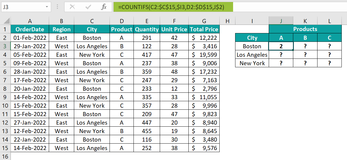
Apply the formula from the J3 cell to all the other cells.

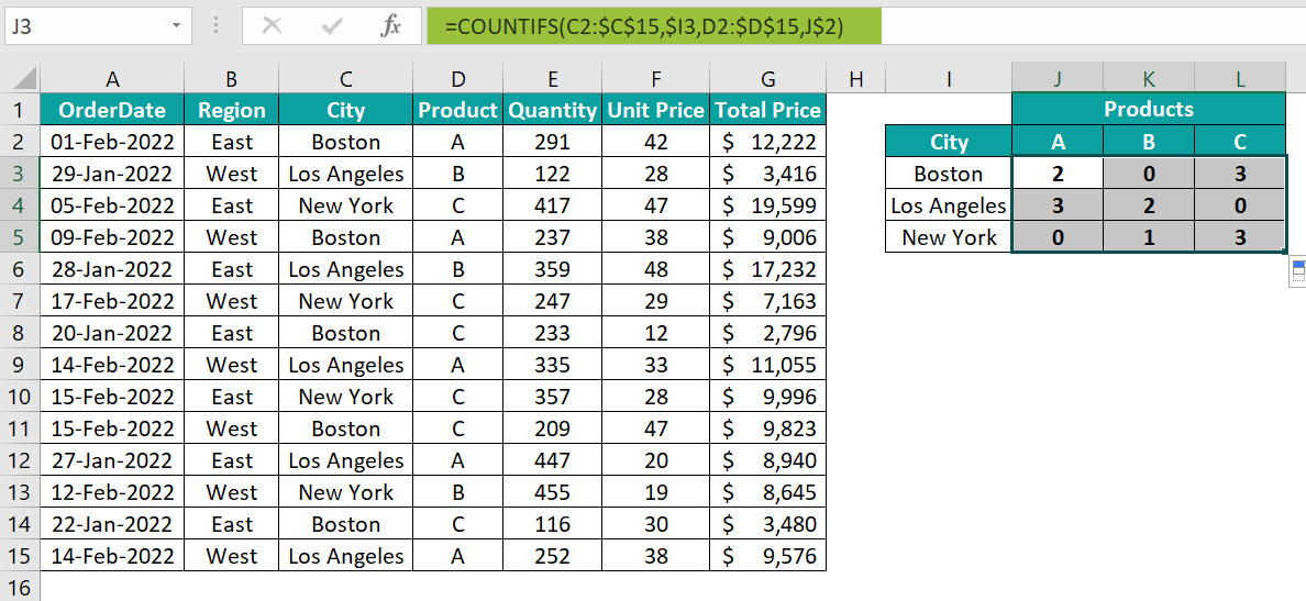
There we have the summary table which shows the count of products sold in each of the cities.

Example #2 – Three Conditions (Multiple Criteria)

With the continuation of the previous example, we will see how to apply 3 conditions with the COUNTIFS function.

The previous summary showed us the count of each product in each city i.e., how many times each product was sold in each city.

• Step 1: Similarly, now we need to apply another condition i.e., Region criteria. Create a drop-down list of regions in cell I1.

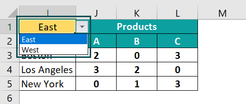
• Step 2: Next, edit the previous formula in cell J3 by pressing the Excel shortcut key F2.

• Step 3: The third criteria we need to give is the “Region” column. Hence, choosing the criteria range 3 from the table from the range B2:B15 and making it an absolute reference by pressing the F4 key once.

• Step 4: Next, choose criteria 3 as I1 where the drop-down of the regions is created after the cell selection makes this an absolute reference by pressing the F4 key once.

• Step 5: Now, all three criteria are given to the COUNTIFS function. The first criterion is City, the second criterion is Product, and the third criterion is Region. Close the bracket and hit the Enter key to get the result. And, apply the formula to all the other cells of the summary table.

• Step 6: The result is zero everywhere. This is because the region criteria cell I1 is blank. We need any one of the regions from the drop-down cell to show up the results.

Now the count is showing only for the region “East”. If we change the region to “West”, it will show count only for the “West” region.

Example #3 – Comparison (Logical) Operators

COUNTIFS function’s versatility is that we can use all kinds of logical operators to apply the criteria. The following logical operators in Excel are commonly used with the COUNTIFS function.

> Greater Than

>= Greater Than or Equal to

< Less Than

<= Less Than or Equal to

= Equal to

<> Not Equal to

Let us look at some examples of applying these logical operators.

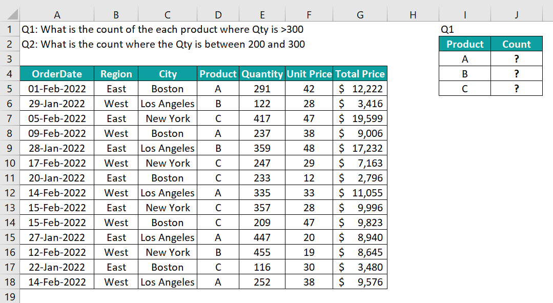
We will use the same data from the previous example and try to solve some of the questions.

The first question that we are trying to answer is as follows:

Q1: What is the count of each product where Qty is >300

• Step 1: We need to find each product’s count when the qty sold is >300. Create a table products table like the following.

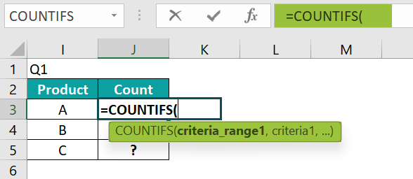
• Step 2: Next, enter the COUNTIFS function in cell J2.

Step 3: Then, choose the criteria to range 1 as the product column.

• Step 4: Choose the criteria as cell I3.

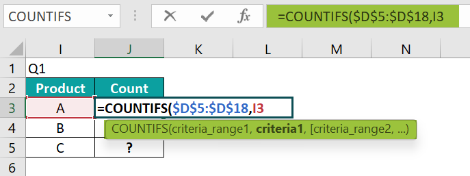
• Step 5: Next, choose the criteria to range 2 from the Qty column.

• Step 6: We need to find the product count where the Qty is >300, so first, we need to provide the logical operator greater than in double quotes followed by the Qty number.

• Step 7: Now, close the bracket and hit the Enter key to get the result.

So, every product is sold 2 times when the Qty is >300.

Now, look at the second question.

Q2: What is the count where the Qty is between 200 and 300

This time we need to find the product count between two qty ranges i.e., between 200 and 300.

• Step 1: First, we need to apply the >=200 logic.

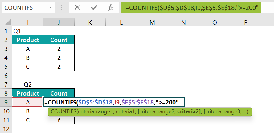
• Step 2: Again, select the Qty column and apply the criteria as <=300.

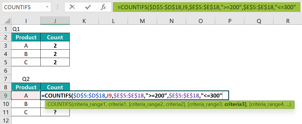
• Step 3: Close the bracket and hit the Enter key to get the result.

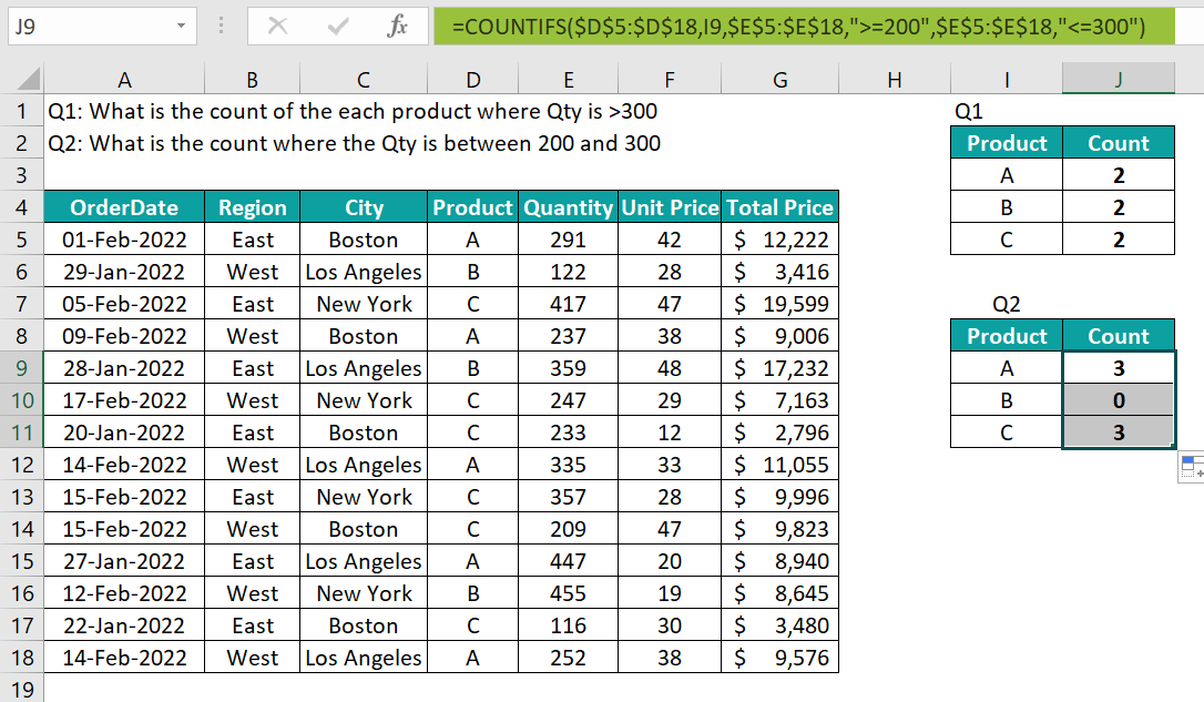
This will give us the count of each product where the qty is between 200 and 300. Product B’s count is zero because no line item is in the range of 200 and 330.

Example #4 – Date Values And Comparison Operators

The COUNTIFS function will allow us to apply logical operators to get the count between two dates.

For example, assume we need to find how many transactions there are between the dates 25^th Jan 2022 and 24^th Feb 2022.

• Step 1: First, set up the criteria cells like the following.

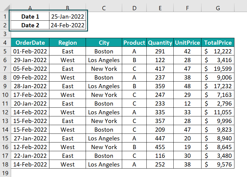
• Step 2: Enter the COUTNIFS function in any of the cells.

• Step 3: For Criteria Range 1, choose the OrderDate column.

• Step 4: Now, we need to enter the criteria; here, we are looking between two dates. So, first, give the logical operator >= in double quotes.

• Step 5: Enter the ampersand (&) symbol and choose the Date1 cell B1.

• Step 6: In criteria range 2, again, we need to select the order date column.

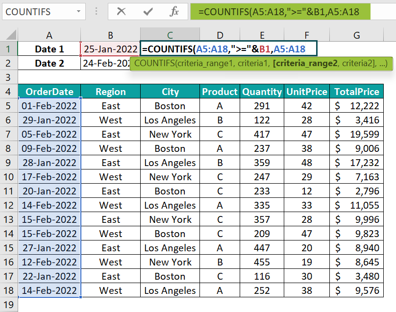
• Step 7: For criteria 2 we need to enter the logical operator <= in double quotes followed by the ampersand (&) symbol and Date 2 cell B2.

• Step 8: Close the bracket and hit the Enter key to get the result.

The total transactions count between the given two dates is 12.

COUNTIFS Excel Function Not Working

If you have applied the COUNTIFS function and if it is not working, there are two possibilities. They are:

#1 – All The Criteria Ranges Should Be The Same

When we select the criteria range for multiple criteria ranges, all the range’s lengths should be the same. For instance, look at the following image.

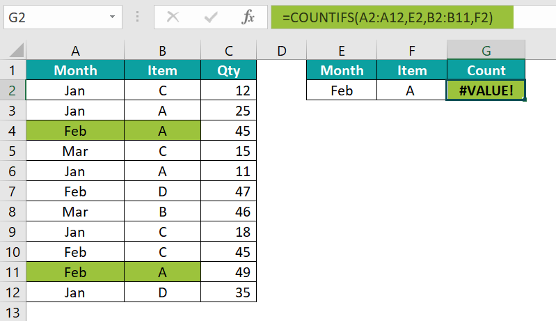
We have applied the COUTNIFS function to get the count of Product A for the month “Feb”. However, there are entries in the data range but the COUNTIFS function is returning the error result i.e., #VALUE! error

The reason for this is two criteria ranges were selected. One is for the Product, and the other one is for the Month.

As we can see month range selection is from A2:A12 but the Item range selection is B2:B11, so there is an inconsistency in the length selected between these two criteria ranges. Hence, the COUNTIF function is returning the error.

#2 – Criteria Value Should Be The Same

There are chances that the criteria value is not the same as the value in the table. For instance, look at the following image.

Again, the same product and same month but this time the count is 0. This is because there is an extra space after the item name “A”.

Because of the extra space character found in the criteria cell F2, the COUNTIFS function was not able to match thus returning the count as zero.

To fix these issues, we use the TRIM excel function before we supply the criteria.

As we can see we have supplied the item criteria cell F2 through TRIM. The TRIM function removed the unnecessary space characters and supplied the accurate value.

Important Things To Note

• The COUNTIFS function will return #VALUE! Error when the criteria range selection is not consistent.
• When we supply the date criteria, the date value should be in the same format as in the data range.
• The COUTNIFS function can take up to 127 criteria ranges and criteria.
• The COUNTIFS function is available in Excel 2007 versions.
• The COUTNIFS function looks for the exact match of the criteria in the given range. If the criteria given are not exact, then it will return the count as 0.

Frequently Asked Questions (FAQs)

Download Template

This article must be helpful to understand the COUNTIFS function in excel, with its formula and examples. You can download the template here to use it instantly.

Recommended Articles

This has been a guide to COUNTIFS Function in Excel. Here we learn how to use the COUNTIFS() function formula with examples and downloadable excel template. You can learn more from the following articles –

• COUNTIF With Multiple Criteria
• COUNTBLANK In Excel
• DCOUNT Excel Function