
What Is EXACT Function In Excel?
The EXACT Function in Excel is used to check whether two strings are the same and returns TRUE or FALSE. The function compares two strings between two cells and returns TRUE if both values are similar & same. Otherwise, it will return FALSE when both strings do not match.
The EXACT Function in Excel is an inbuilt function of Excel that is categorized under the ‘TEXT’ function of ‘Function Library.’ This is case-sensitive when looked up between two strings.
Use this EXACT Function in Excel Template to follow along with the examples in this article.
Download Excel TemplateFor example, consider the below table to detect the exact values in cells A1 and B1. We need to use the below steps to obtain the result with EXACT function.

The steps used to detect the exact values in Excel are as follows:
Step 1: Select the cell to display the result. In this example, we have selected cell C1.
Step 2: Enter the EXACT function formula in cell C1.
The complete formula is =EXACT(A1:A2,B1).
Step 3: Press Enter key.
We can clearly see that the function has returned the value as TRUE in cell C1.

Similarly, we can use the function to fetch the exact value.
Key Takeaways
- The Excel EXACT Function returns false value if there is a difference in case pattern between text strings, i.e., sentence case, lowercase, uppercase, proper case & toggle case.
- The excel EXACT formula is =EXACT(text1,text2).
- The function can only compare and finds the match for string values.
- It converts the numeric values as parameters to text.
- The EXACT function is in Excel for Office 365, Excel 2019, Excel 2016, Excel 2013, Excel 2011 for Mac, Excel 2010, Excel 2007, Excel 2003, Excel XP, and Excel 2000.
EXACT() Excel Formula
The syntax of the EXACT Excel Formula is

where,
- text1: It specifies the first string for which we want to check the exact match.
- text2: It indicates the second string against which we want to test.
Unlike other functions, both the arguments are mandatory.
How To Use EXACT Excel Function?
We can insert the function with the following 2 methods.
Method #1 – Access From The Excel Ribbon
- Choose the empty cell which will contain the result.
- Go to the Formulas tab and click it.
- Select the Text option from the menu.
- Select EXACT from the drop-down menu.
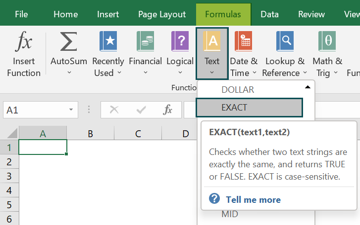
- A window called Function Arguments appears.
- As the number of arguments, enter the value in the text1 & text2.
- Select OK.

Method #2 – Enter The Worksheet Manually
- Select an empty cell for the output.
- Type =EXACT( in the selected cell. Alternatively, type =E and double-click the EXACT function from the list of suggestions shown by Excel.
- Press the Enter key.
Let us look at an example to learn about this function.
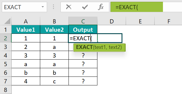
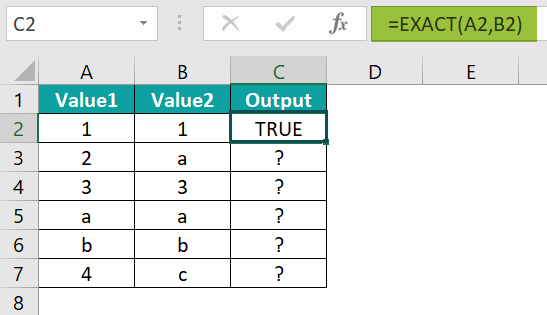
The below table shows values in columns A and B. We need to use the below steps to calculate exact values with Excel EXACT Function.

The steps to evaluate the values using Excel EXACT Function are as follows:
- To begin with, select the cell where we will enter the formula and calculate the result. The selected cell, in this case, is cell C2.
- Next, we will enter the EXACT formula in cell C2.

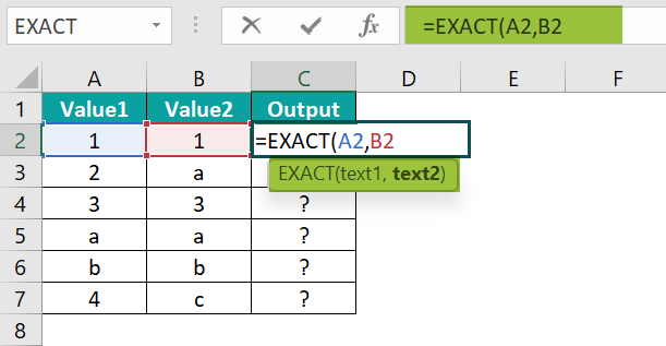
- Then, enter the value of ‘text1’ as A2, i.e., the first text value.
- Similarly, enter the value of ‘text2’ as B2, i.e., the second text value.
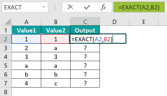
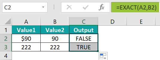
- The complete formula is =EXACT(A2,B2) in cell C2.

- Next, press Enter key.
Then, the function is returned as TRUE in cell C2 as shown in the image below.
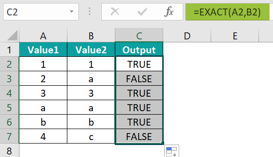
- Drag the cursor to cell C7, as shown in the following image.
Likewise, using Excel EXACT Function, we can find exact values in excel.

Examples
Example #1
The following table depicts the values containing spaces in columns A and B. We need to use the below steps to calculate the day with Excel EXACT Function.
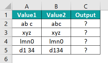
The steps to evaluate the values with the function are as follows:
Step 1: First, select the cell where we will enter the formula and calculate the result. The selected cell, in this case, is cell C2.
Step 2: Next, we will enter the Excel EXACT formula in cell C2.
Step 3: Then, enter the value of ‘text1’ as A2, i.e., the first text value.
Step 4: Enter the value of ‘text2’ as B2, i.e., the second text value.
Step 5: The complete formula is =EXACT(A2,B2) in cell C2.
Step 6: Then, press Enter key.
The result is shown in cell C2 as FALSE in the image below.
Step 7: Drag the cursor to cell C5, as shown in the following image.

Similarly, we can use the function to fetch the exact values.
Example #2
The following table shows the values containing different formats. We will check the exact match between the values with EXACT function in Excel.

The steps to evaluate the values with excel EXACT Function are as follows:
Step 1: To begin with, select the cell where we will enter the formula and calculate the result. The selected cell, in this case, is cell C2.
Step 2: Next, we will enter the excel EXACT formula in cell C2.
Step 3: Enter the value of ‘text1’ as A2, i.e., the first text value.
Step 4: Enter the value of ‘text2’ as B2, i.e., the second text value.
Step 5: The complete formula is =EXACT(A2,B2) in cell C2.
Step 6: Press Enter key.
The function has returned the result in cell C2 as ‘FALSE’.
Step 7: Drag the cursor to cell C3, as shown in the following image.
Likewise, we can find exact values with EXACT Function.
Example #3
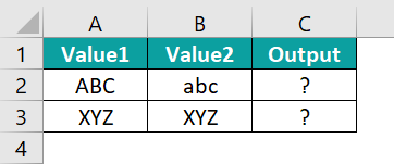
The below table depicts the values containing different cases of string in columns A and B. We will check the exact match between the values with Excel EXACT function.
The steps to evaluate the values by the EXACT Function in Excel are as follows:
Step 1: Select the cell where we will enter the formula and calculate the result. The selected cell, in this case, is cell C2.
Step 2: Next, we will enter the EXACT formula in cell C2.
Step 3: Enter the value of ‘text1’ as A2, i.e., the first text value.
Step 4: Enter the value of ‘text2’ as B2, i.e., the second text value.
Step 5: The complete formula is =EXACT(A2,B2) in cell C2.
Step 6: Press Enter key.
The result is shown in cell C2 as FALSE.
Step 7: Drag the cursor to cell C3, as shown in the following image.

Similarly, we can use the function to find the exact values.
Important Things To Note
- The EXACT function is used to find the exact values in the given table or range. It is case-sensitive, and therefore, capital letters are not equal to small letters.
- Unlike other functions, both the arguments in Excel EXACT function formula are mandatory.
- The EXACT function is very easy to use and is simple to work with two arguments.
- The standard equal to the “=” operator is not case-sensitive.
- The EXACT Function in excel ignores the formatting difference between the two cells.
Frequently Asked Questions (FAQs)
The EXACT function matches the exact value of some data with another in Excel. This is the special function to compare two strings and states whether they are an exact match or not. The function is case-sensitive function that compares two text values and returns Boolean True or False.
The syntax of the EXACT function is
=EXACT(text1,text2)
The EXACT Function in Excel will not work if the table array entered as the argument is a group of different columns, not of the same column.
For example, the below table shows the values in different columns as entered in an array which generates an error, and we will check the match using EXACT function.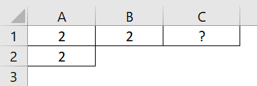
The steps to evaluate the values by the Excel EXACT Function are as follows:
• Step 1: First, select the cell where we will enter the formula and calculate the result. The selected cell, in this case, is cell C1.
• Step 2: Next, we will enter the EXACT formula in cell C1.
• Step 3: Then, enter the value of ‘text1’ as A1:B1, i.e., the first text value.
• Step 4: Enter the value of ‘text2’ as A2, i.e., the second text value.
• Step 5: So, the complete formula is =EXACT(A1:B1,A2)in cell C1.
• Step 6: Press Enter key.
Clearly, we can see that the function has returned the results in cell C1 as the “#VALUE!” error.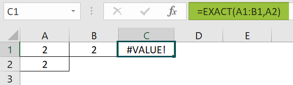
Similarly, we can use Excel EXACT function to find the exact values.
We can insert Excel EXACT Function using the following steps:
• Choose the empty cell which will contain the result.
• Go to the Formulas tab.
• Select the Text option from the menu.
• Select EXACT from the drop-down menu.
• A window called Function Arguments appears.
• As the number of arguments, enter the value in the text1 & text2.
• Select OK.
Use this EXACT Function in Excel Template to follow along with the examples in this article.
Download Excel Template