Excel Reverse Order

What Is Reverse Order In Excel?

Excel reverse order involves flipping the data in a column, with the values at the bottom, in the original data, showing at the top after the flip. Though Excel does not offer an inbuilt option to reverse the order of data rows, one can flip the data using the Sort option, Excel formula, and VBA coding technique.

Users can use this Excel option to reverse the order of unsorted data, such as names and numeric values in a column or array.

For example, the table below contains a list of employee names.

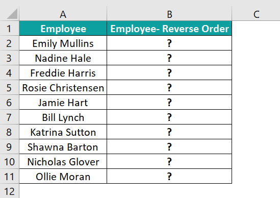
Suppose the requirement is to reverse the order of the employee names and display the output in column B.

Then, we can reverse order of cells in Excel column A using the INDEX and ROWS functions in the target cells and achieve the desired outcome.

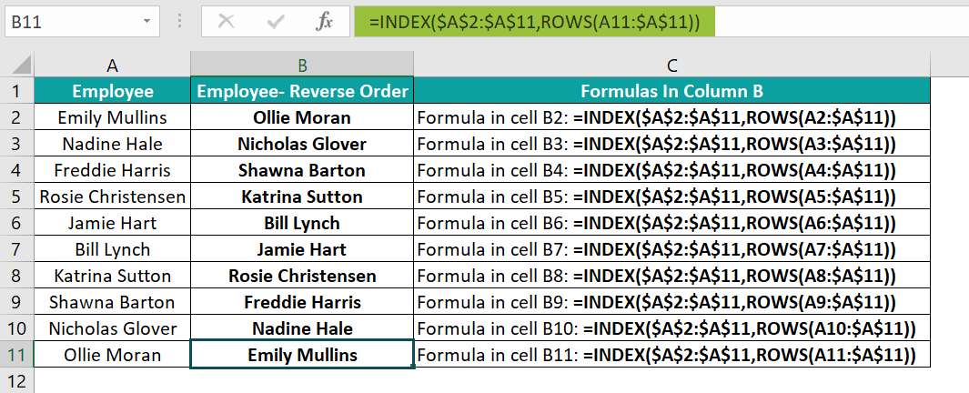
In the above Excel reverse name order example, the ROWS() returns the number of rows in the specified column A range. And then, the INDEX() returns the value in the cell at the intersection of the specified column range and the count of rows the ROWS() returned.

What Is Reverse Order In Excel?

Excel reverse order is a feature to display the given data in a column flipped or the top-to-bottom order of the data reversed.
The option helps users to sort and display the data, such as numbers and texts, in reverse order.
Though Excel can sort the given data in ascending and descending orders, it does not have the option to reverse the order of the data rows directly. However, we can use the Sort option, VBA coding, and Excel formulas containing the INDEX and ROWS functions to achieve the desired reverse order of data.

Explanation

Excel offers an inbuilt function, Sort, to arrange the data in ascending or descending order.

However, in some scenarios, we may require to flip the given columns of data, vertically or horizontally, with the data remaining unsorted. For example, we may need to only display a list of items in reverse order without sorting them alphabetically.

We can apply the below-explained methods to use the Excel reverse order feature in such cases.

Excel VBA – All in One Courses Bundle (35+ Hours of Video Tutorials)

If you want to learn Excel and VBA professionally, then Excel VBA All in One Courses Bundle (35+ hours) is the perfect solution. Whether you’re a beginner or an experienced user, this bundle covers it all – from Basic Excel to Advanced Excel, Macros, Power Query, and VBA.

Start Learning Now

How To Reverse The Order Of Data Rows In Excel?

We can achieve the Excel reverse order of data rows using the following three ways:

The Sort option from the Data tab
Excel formula containing the INDEX() and ROWS()
VBA code

The following illustrations explain the above mentioned methods to vertically flip the data in one or more columns.

And while the Sort and the VBA coding options can reverse and display the flipped data in the same column, the Excel formula can show the flipped data in another column.

Example #1 – Using Simple Sort Method

We can reverse order of cells in Excel columns vertically using the sort method.

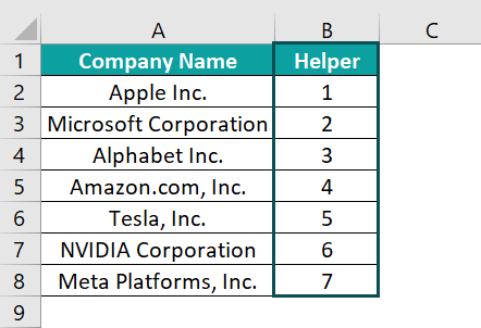
For example, the following table contains a set of top tech US companies.

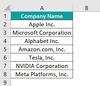
How to Use Reverse Order in Excel - Example 1 - Using Simple Sort Method

Suppose the requirement is to flip the order of the cells in column A. Then, we can perform the required Excel reverse name order operation using the Sort option.

Step 1: Add a helper column, with numbers in ascending order, to the source data, as depicted below.

Example 1 - Using Simple Sort Method - Step 1

Step 2: Next, select the entire data range (with or without the column headers) and then, click Data → Sort to open the Sort window.

Example 1 - Using Simple Sort Method - Step 2

Alternatively, we can select the data range and press the shortcut keys Alt + D + S to open the Sort window.

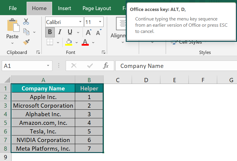
Example 1 - Using Simple Sort Method - Step 2a

Pressing the last key in the keyboard shortcut S will open the Sort window.

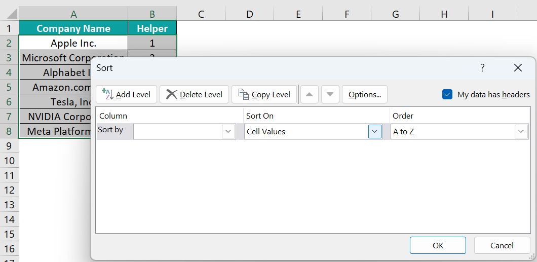
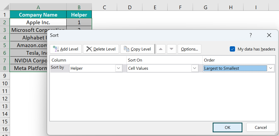
Example 1 - Using Simple Sort Method - Step 2b

Step 3: Set Sort by as Helper.

Example 1 - Using Simple Sort Method - Step 2c

And pick the option Largest to Smallest as the Order.

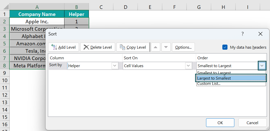
Example 1 - Using Simple Sort Method - Step 2d

Finally, click OK to close the window.

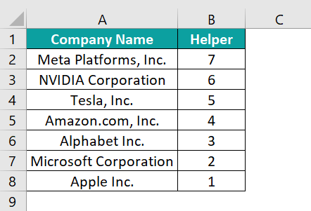
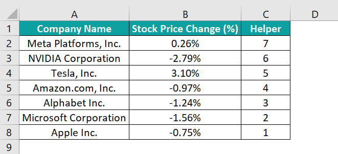
Example 1 - Using Simple Sort Method - Step 2e

And the required Excel reverse order of data will appear as depicted below. We see the company names are in reverse order.

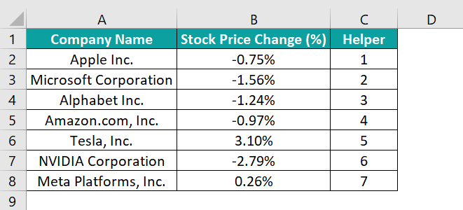
Example 1 - Using Simple Sort Method - Step 2f

On the other hand, suppose the original data includes two columns, as shown below.

Example 1 - Using Simple Sort Method - Step 2g

And if we aim for Excel reverse column order, row-wise, for the entire data, then, we can follow steps 1 to 3, explained above, to achieve the required outcome.

Otherwise, we can add the helper column with numbers in ascending order and use the following steps to get the required Excel reverse order of list in each source column.

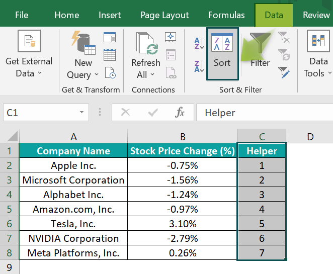
Example 1 - Using Simple Sort Method - Step 2h

Step 1: First, select the Helper column data (with or without the column header) and follow the path Data → Sort Z to A to sort the Helper column data in descending order.

Step 2: Next, we will see the Sort Warning message, where we must select the option to expand the selection.

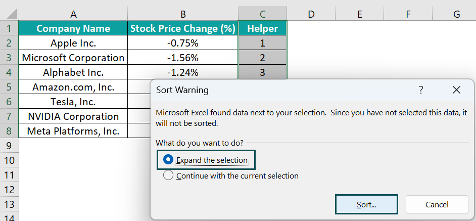
And clicking Sort in the warning dialog box will flip the three columns’ data vertically, as depicted below.

We can also follow the above-explained alternative method in the first scenario, with the source data containing one column of data to reverse.

Example #2 – Using Excel Formula

Using the INDEX and ROWS functions, we can apply the Excel reverse order feature.

For example, the following table contains an item list.

Suppose we require the Excel reverse order of list, given in column B in column C.

Then, here is how to use the INDEX and ROWS functions in the target cells to obtain the required output.

Step 1: Select cell C3, enter the below formula, and press Enter.

=INDEX($B$3:$B$11,ROWS(B3:$B$11))

Step 2: Next, using the excel fill handle, implement the formula in cell range C4:C11.

Let us see the cell C3 expression to understand how the formula works. First, the ROWS() returns the number of rows in the range B3:$B$11, which is 9. And then, the INDEX excel formula returns the value in the cell where the column range B3:B11 and row 9 meet, which is the cell B11 value, Baking Powder.

Likewise, the Excel reverse order formulas list the column B items in column C, with their order flipped.

Example #3 – Using VBA Coding

We can apply the Excel reverse order option from the VBA Editor. Let us see the steps with an example.

The table below contains a list of company codes and their volumes.

And we need to achieve Excel reverse column order for the above data and display the outcome in column B.

Then, the steps are as follows:

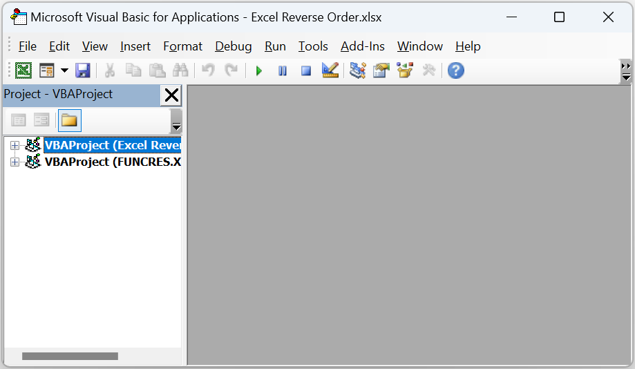
Step 1: First, open the worksheet containing the above table and then, click Alt + F11 to access the VBA Editor window.

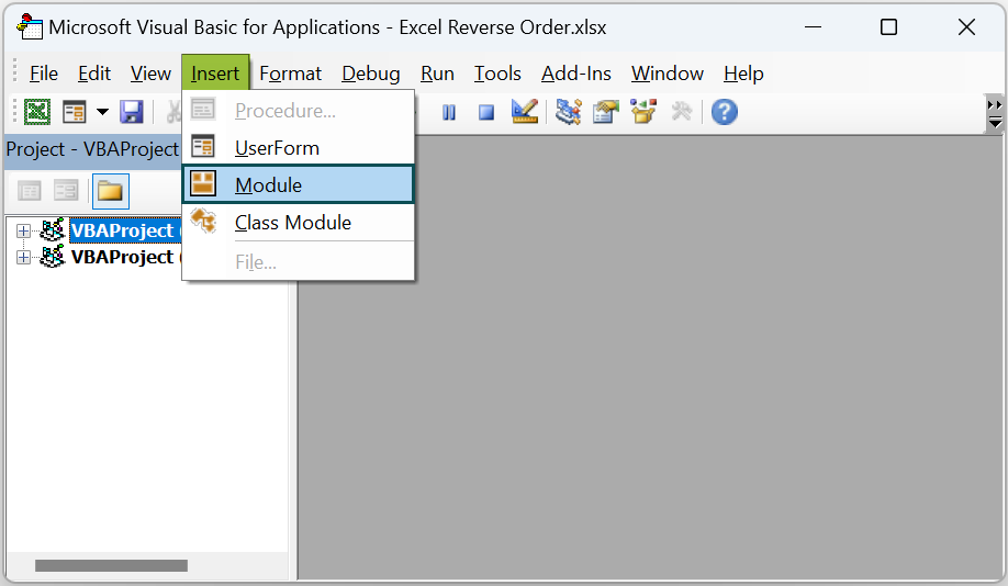
Step 2: Pick the applicable VBAProject and choose the Module option from the Insert tab to open a new module window, Module1.

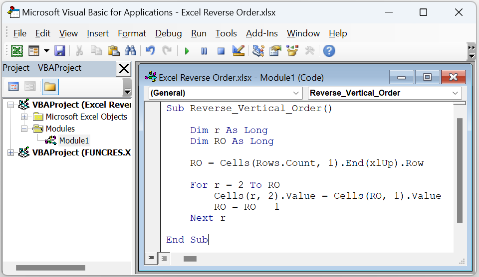
Step 3: Next, enter the VBA code to achieve Excel reverse order of the given data in the target cells.

Sub Reverse_Vertical_Order()

Dim r As Long

Dim RO As Long

RO = Cells(Rows.Count, 1).End(xlUp).Row

For r = 2 To RO

Cells(r,2).Value = Cells(RO, 1).Value

RO = RO – 1

Next r

End Sub

Step 4: Click the play icon in the menu to run the VBA code.

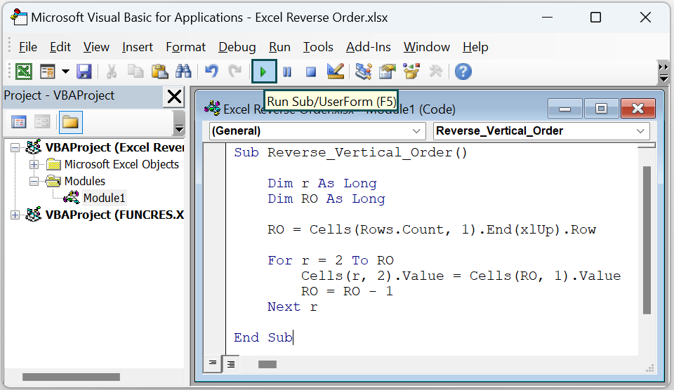
We can now go to the active worksheet to view the given data in the reverse order in column B.

First, we declare two Long variables, r, and RO. While r is the counter variable for the For loop, RO gets the last row count in the worksheet containing data, which is 7.

Next, the For loop starts assigning the column A cell values from the bottom to column B cells to fill the column from the top. The process continues till the counter reaches the last row, 7. And thus, the loop fills all column B cells till row 7, with the given data appearing in reverse order.

Important Things To Note

When using the Sort option from the Data tab to achieve Excel reverse order of data rows, ensure the Sort Options has the default setting of Sort top to bottom. It will maintain the sorting orientation as Column to reverse the data order vertically.
When using the helper column while applying the Sort option to flip a column of data, ensure the numbers in the helper column are in ascending order.

Frequently Asked Questions (FAQs)

1. Can I flip columns and rows in Excel?

We can flip columns and rows in Excel.

If we have to flip columns or rows of data, use the Sort option from the Data tab.

And if we must flip columns and rows to rows and columns respectively, use the Transpose excel option from the Paste Special window.

2. How to reverse order in Excel horizontally?

We can reverse order in Excel horizontally using the following steps.
1) First, change the given data rows into columns using the Transpose option in the Paste Special window.
2) Next, sort the columns using the Sort option from the Data tab.
3) Finally, rotate the columns to rows using the Transpose option in the Paste Special window.

Let us see the steps with an example.

The below table shows a set of fruits, their order dates, and order status data.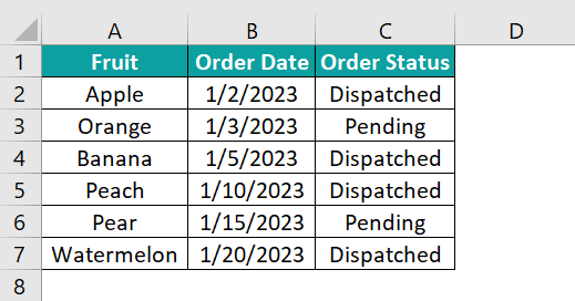

Suppose the requirement is to flip the data order horizontally. Then, the steps are as follows:

• Step 1: Select the table range and press Ctrl + C to copy the data.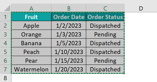

Select a cell, say, cell E1, press the shortcut keys Alt + E + S to open the Paste Special window, and check the Transpose box.

Clicking OK will paste the transposed data into the selected cell.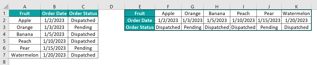

• Step 2: Add a helper column of numbers in ascending order to the end of the transposed data in column L.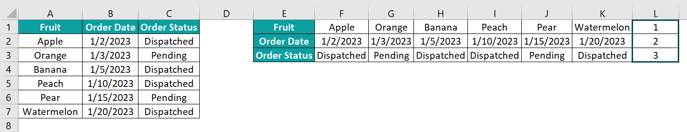

• Step 3: Click on a cell in the transposed data range and follow the path Data → Sort to open the Sort window.

• Step 4: Ensure the My data has headers box remains unchecked and pick column L, the helper column, as the Sort by option.

And pick the Largest to Smallest option as the Order.

Clicking OK will reverse the order of the values in the transposed data.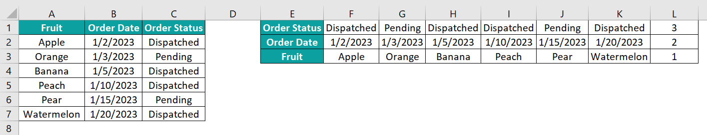

• Step 5: Select the transposed data range, leaving the helper column unselected. And press Ctrl + C to copy the data.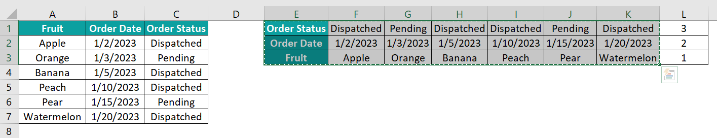

Select a cell, say, cell A10, press the shortcut keys Alt + E + S to open the Paste Special window, and check the Transpose box.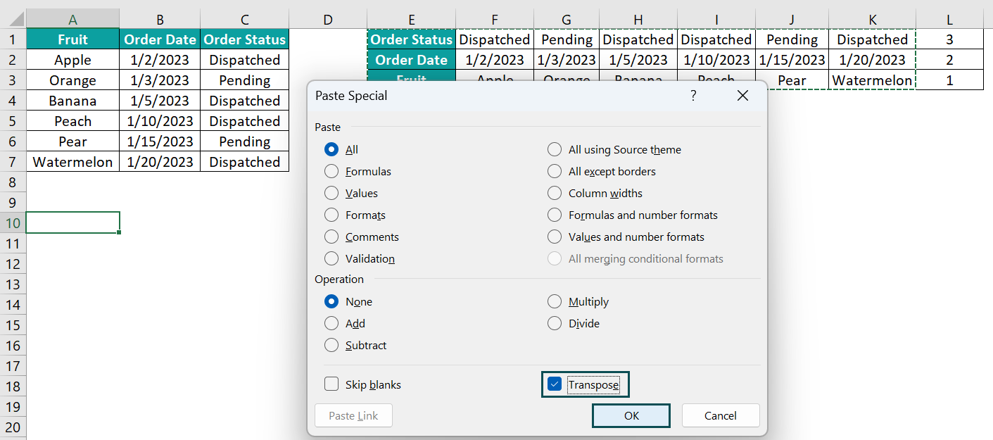

And clicking OK will flip the source data horizontally.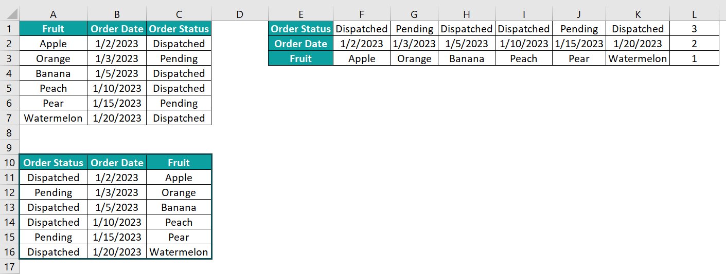

When we compare the source and the final data, the order of the data in each row appears flipped horizontally in the output.

3. Why is reverse order in Excel not working?

The reverse order in Excel is not working, perhaps because of the below reasons:
• We tried applying the Sort method without the numbers in the helper column being in ascending order.
• The Sort Options setting in the Sort window does not match the desired reverse order type (vertical and horizontal).

Download Template

This article must be helpful to understand the Excel Reverse Order, with its formula and examples. You can download the template here to use it instantly.

Excel Reverse Order Download

Excel Reverse Order