
What Is TRANSPOSE In Excel?
TRANSPOSE in Excel is a function to rotate (switch) data from rows to columns and vice versa. It is a part of the LOOKUP and reference functions. In addition, the TRANSPOSE function helps users sort unformatted data in the desired format.
TRANSPOSE function in Excel also converts the range of table array from vertical to horizontal and vice versa. Its formula is:
Use this TRANSPOSE In Excel Template to follow along with the examples in this article.
Download Excel Template=TRANSPOSE(array)
For example, the following image shows the array of three numbers 10, 20, and 30 as input in row 2. We will transpose the table data into column E with the TRANSPOSE formula.
- Select the empty cell E2:E4.
- Type the formula =TRANSPOSE(A2:C2).
- Press CTRL+SHIFT+ENTER.
The output is 10, 20, and 30 in column E as a vertical representation.
Key Takeaways
- The TRANSPOSE option in Excel is used to switch rows and columns. It is a part of the Reference functions in Excel. Its syntax is =TRANSPOSE(array)
- Since it is a dynamic array formula, after inputting the formula and selecting the array, press Ctrl+ Shift+ Enter.
- The TRANSPOSE function in Excel converts blank cells to zeros.
Syntax Of TRANSPOSE() In Excel
The following image shows the syntax of the TRANSPOSE() in excel:
- array = This is the range of cells to be transposed.
How To TRANSPOSE In Excel?
Transposing Excel data can be tricky and difficult. There are three approaches to TRANSPOSE Excel data. Let us look at those along with examples to understand how to use the TRANSPOSE formula:
1. Paste Special
It is quick and easy to use. However, this approach is best used when you want to transpose data as a one-off action and do not need to transpose data repeatedly for months, weeks, or days.
The following image depicts the Roll Number, Names, and Marks of 7 art students in a vertical table array. Next, we need to transpose the vertical table data into a horizontal data table with the Paste Special Transpose method.
In the table, the data is reflected as below:
- Column A shows Roll Number
- Column B contains the Names of the students
- Column C contains Marks of the students
Let us look at the step-by-step explanation of the Paste Special Transpose approach:
- Step 1: Select the table array range A2:C9, which is to be transposed.
- Step 2: Right-click and click “Copy.”
- Step 3: Select the empty cell F2, where you want to transpose the data.
- Step 4: Right-click and click “Paste Special.”
- Step 5: The “Paste Special” window pops up. The shortcut key for opening the “Paste Special” window is CTRL+ALT+V.
- Step 6: Select the checkbox “Transpose” and click “OK“
- Step 7: The output comes as follows in the cells F2:M4.
Therefore, the horizontal data table is transposed into the vertical data table.
2. TRANSPOSE Function
The TRANSPOSE function in Excel shifts data from horizontal to vertical representation and vice versa. This function is very simple to understand. It takes only one table array which you want to transpose.
Syntax of TRANSPOSE in Excel
- array = This is the range of cells to be transposed.
Example #1
The following image depicts a company’s invoice, featuring Invoice ID, Date, Unit Price, Tax, and Total Price in a vertical table array. Next, we must transpose the vertical data table into a horizontal data table with the TRANSPOSE function.
In the table, the data is reflected as below:
- Column A shows Invoice ID
- Column B contains the Date
- Column C contains the Unit Price of the products
- Column D contains the Tax amount
- Column E contains the Total amount.
- Step 1: Select the empty cell H1:M5.
Step 2: Type the formula =TRANSPOSE(A2:E7).
Step 3: Press CTRL+SHIFT+ENTER.
The output comes as follows in the cells H1:M5 as the horizontal representation.
Therefore, the horizontal data table is transposed into the vertical data table.
Note: It returns the #VALUE! error if the number of rows is not equal to the number of columns and rows of the source data.
Example #2
The following image depicts the company’s employee ID, Names, and Salary in a horizontal table array. We need to transpose the horizontal data table into a vertical one with the TRANSPOSE function.
In the table, the data is reflected as below:
- Row 1 shows Emp. ID
- Row 2 contains Emp. Name
- Row 3 contains the Annual Salary of the employees
- Step 1: Select the empty cell A6:C11.
- Step 2: Type the formula =TRANSPOSE(B1:G3).
Step 3: Press “CTRL + SHIFT + ENTER”.
The output comes as follows in the cells A6:C11 as the vertical representation.
Therefore, the vertical data table is transposed into the horizontal data table.
3. Power Query Tool
It is a method of choice when we repeatedly get data from the same source, and we need to transpose it. Also, it is a quick and powerful tool.
The following image depicts sales of textile business in Europe, Asia, and North America. First, we need to transpose the horizontal data table into a vertical one using the Power Query Tool method.
In the table, the data is reflected as below:
- Row 1 shows Sales by Region
- Row 2 contains the total sales revenue in Europe
- Row 3 contains the total sales revenue in Asia
- Row 4 contains the total sales revenue in North America
Let us look at the step-by-step explanation of the Power Query Tool approach:
- Step 1: Select the data table array B1:F4 to be transposed.
- Step 2: Click the “Data” tab.
Step 3: Select “From Table/Range” under the “Get & Transform Data” option.
- Step 4: The “Create Table” dialogue box opens. Enter the table array range $B$1:$F$4.
- Step 5: Then, the “Query Editor” dialogue box opens.
- Step 6: Select the “Transform” tab.
Step 7: In the “Use First Row As Headers” selection, choose the “Use Headers As First Row” option. This ensures that the table’s header is treated as a part of the data and transposed.
Step 8: Then click the “Transpose” option.
Step 9: Go to the “File” tab, and click the “Close & Load” option.
Step 10: The transposed data is now loaded on the new sheet of the same workbook.
It can also be used with the LOOKUP function in Excel.
Important Things To Note
- The TRANSPOSE function links data to the source.
- The formula only copies values, not the data format.
- It is an array function, so users need to use CTRL+SHIFT+ENTER, not just the ENTER.
- The result cannot be changed once the function is entered into the cell. Instead, the whole array needs to be deleted to change.
- The function can be combined with IF Function, CONCATENATE Function, INDEX function, MATCH Function, etc.
- It can also be used with the LOOKUP function in Excel.
- The TRANSPOSE function accepts the mandatory argument, “array.”
- It is very easy to use in Microsoft 365, and the results will automatically come up as an array of values.
- If you want the transposed results to update when you change the source data, you need to type the TRANSPOSE formula into the cell where you want the transposed data. The data will flow down and to the right of the cell with the formula; no need to copy and paste.
- The TRANSPOSE function is dynamic. The result data automatically changes when the changes are done in the source data table.
Frequently Asked Questions (FAQs)
Transpose means two or more things changing their places with each other. For example, the TRANSPOSE in Excel formula flips data of the table array from horizontal to vertical and vice versa.
=TRANSPOSE(array)
The TRANSPOSE function changes the position of data, like the first row of the array becomes the first column, the second row becomes the second column, and so on. Only cell values are copied and shifted.
You can locate the TRANSPOSE function in Excel using the following steps:
1. Copy the cell range of the table array.
2. Select the empty cell where you want to paste the data.
3. Right-click and select the “Paste Special.”A window pops up of “Paste Special.”
4. Select the checkbox of “Transpose” under the “Operation” option.
5. Click OK.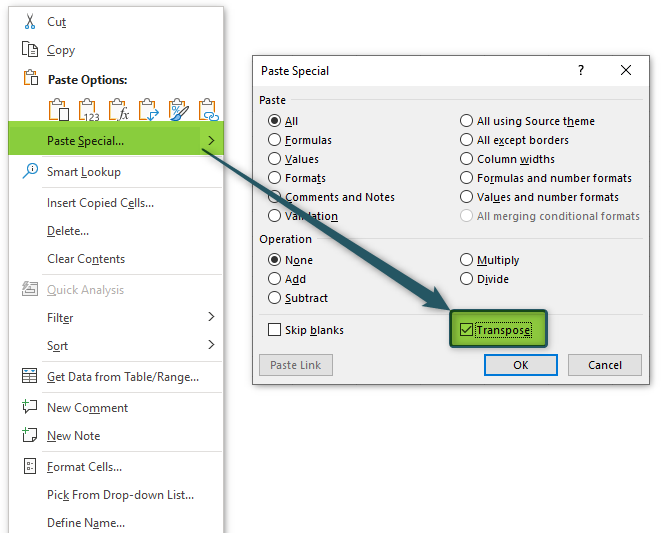
Here is the step-by-step representation of how the TRANSPOSE function transposes the cell content:
1. Select a blank cell.
2. Type the formula =TRANSPOSE(array)
3. Select the range of the table array which you want to transpose).
4. Press CTRL+SHIFT+ENTER.
For example, the following image shows the table array of alphabets – aa, bb, cc, and dd as input in the column. We will transpose the data from horizontal representation into a row representation with the TRANSPOSE formula.
• Select the empty cells D2:G2 where we want to transpose data.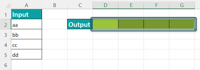
• Type the formula =TRANSPOSE(A2:A5).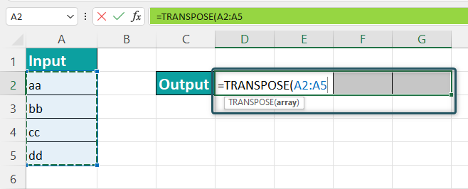
• Press CTRL+SHIFT+ENTER.
• The Output comes as aa, bb, cc, and dd in a row as a horizontal representation.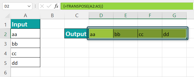
Use this TRANSPOSE In Excel Template to follow along with the examples in this article.
Download Excel Template