What Is Formula Auditing Tools In Excel?
The Formula Auditing Tools in Excel help users to view or troubleshoot the calculations or formula results in a given dataset because we use the function, formulas, and Macros in Excel.
The Formula Auditing Tools are Excel inbuilt features categorized under the Formula Auditing group of the Formula tab.
📥Download the ready-to-use Excel template to practice this tutorial yourself.
Formula-Auditing-Tools-in-ExcelTable of contents
Key Takeaways
- Formula Auditing Tools in Excel allow users to trace the cell references of formulas, dependent cell, view and evaluate formulas, and troubleshoot errors to fix the formulas.
- A Precedent cell is referenced by another cell in a formula, while a dependent cell has its formula.
- An error occurs when a formula does not return a valid result. To view and troubleshoot the error, we can use the Error Checking option.
- The keyboard shortcut is “ALT + M + K + K” to check for errors on a worksheet.
How To Use Formula Auditing Tools In Excel?
We can use the Formula Auditing Tools in Excel as follows:
Choose any cell that is a result of a formula – select the “Formulas” tab – go to the “Formula Auditing” group – select any of the required 6 options, as shown below.

As shown in the above image, there are six built-in Formula Auditing Tools in Excel, namely:
- Trace Precedent – Highlights the cell references in excel of the given formula.
- Trace Dependents – Traces the cell value that is dependent on the selected cell.
- Remove Arrows – Clears the displayed arrows of the formula cell reference.
- Show Formulas – Displays all the formulas used in the worksheet.
- Error Checking – Provides options such as Error Checking, Trace Error, and Circular References in excel, and
- Evaluate Formula – Displays the evaluation of the formula using the BODMAS technique.
We will consider each tool in detail with examples in the Basic Example and the Example sections.
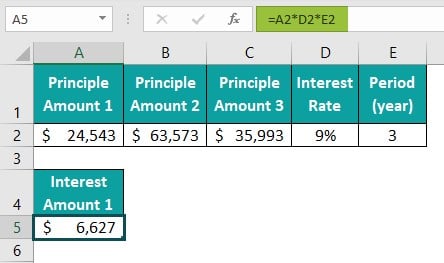
For instance, Mr. Raj has invested in the company’s bond in three Principal Amounts, the interest rate is 9%, and the period is three years. We will first calculate the interest amount, and then Trace Precedents using the Formula Auditing Tool.
In the table, the data is,
- Column A contains Principal Amount 1.
- Column B contains Principal Amount 2.
- Column C contains Principal Amount 3.
- Column D contains the Interest Rate.
- Column E contains Period.

The steps to Trace Precedents using the Formula Auditing Tools are as follows:
Step 1: First, select an empty cell A5, to calculate the interest loan amount, enter the formula =A2*D2*E2, and press the “Enter” key. The result is ‘$6,627’, as shown below.
Step 2: Next, choose cell A5, i.e., the containing the formula – select the “Formulas” tab – go to the “Formula Auditing” group – select the “Trace Precedents” option, as shown below.
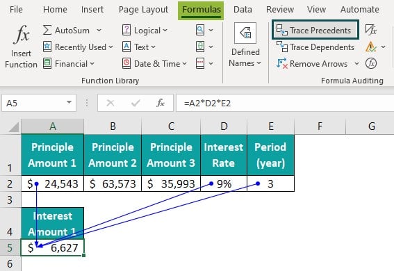
The moment we click the Trace Precedents, the arrows appear, pointing to the cell references of the selected formula cell, as shown above.
Examples
We will now see the remaining six built-in Formula Auditing Tools in Excel with examples.
Example #1 – Trace Dependents
Mrs. Terence has invested in the XYZ company in three Principal Amounts, the interest rate is 34%, and the period is three years. We will first calculate the interest amount, and then Trace Dependents using the Formula Auditing Tool.
In the table, the data is,
- Column A contains Principal Amount 1.
- Column B contains Principal Amount 2.
- Column C contains Principal Amount 3.
- Column D contains the Interest Rate.
- Column E contains Period.

The steps to Trace Dependents using the Formula Auditing Tools are as follows:
1: First, select an empty cell A5, to calculate the interest loan amount, enter the formula =B2*D2*E2, and press the “Enter” key. The result is “$3,53,31,109”, as shown below.

2: Next, choose cell A5, i.e., the containing the formula – select the “Formulas” tab – go to the “Formula Auditing” group – select the “Trace Dependents” option, as shown below.
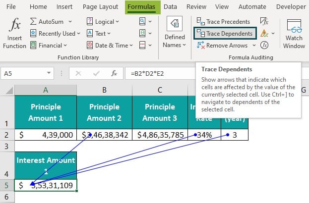
When we click the Trace Dependents, the arrows, appear tracing the cell values that are dependent on the selected cell, as shown above.
Example #2 – Remove Arrows
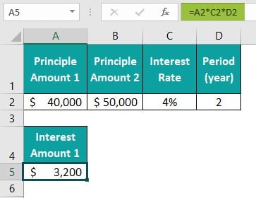
The investors have invested in the company in two Principal Amounts, the interest rate is 4%, and the period is two years. We will first calculate the interest amount, Trace Precedents, and then Remove Arrows using the Formula Auditing Tool.
In the table, the data is,
- Column A contains Principal Amount 1.
- Column B contains Principal Amount 2.
- Column C contains the Interest Rate.
- Column D contains Period.

The steps to Trace Precedents and Remove Arrows using the Formula Auditing Tools are as follows:
1: First, select an empty cell A5, to calculate the interest loan amount, enter the formula =A2*C2*D2, and press the “Enter” key. The result is ‘$3,200’, as shown below.
2: Next, choose cell A5, i.e., the containing the formula à select the “Formulas” tab à go to the “Formula Auditing” group à select the “Trace Precedents” option, as shown below.

3: Finally, to remove the arrows drawn by Trace Precedents, select the “Formulas” tab – go to the “Formula Auditing” group – select the “Remove Arrows” option, as shown below.
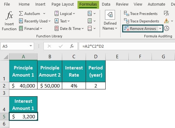
The moment we click the Remove Arrows, the arrows disappear, as shown above.
Example #3 – Show Formulas
Mr. Bond has invested in the company in three Principal Amounts, the interest rate is 2%, and the period is three years. We will first calculate the interest amount, and then use the Show Formula option from the Formula Auditing Tool to view the formula.
In the table, the data is,
- Column A contains Principal Amount 1.
- Column B contains Principal Amount 2.
- Column C contains Principal Amount 3.
- Column D contains the Interest Rate.
- Column E contains Period.

The steps to Show Formulas using the Formula Auditing Tools are as follows:
1: First, select an empty cell A5, to calculate the interest loan amount, enter the formula =A2*$D$2*$E$2, and press the “Enter” key. The result is ‘$3,600’, as shown below.

2: Drag the formula from cell A5 to C5 using the excel fill handle. The output is shown below.

3: Next, choose the cells having formulas, A5:C5 – select the “Formulas” tab – go to the “Formula Auditing” group – select the “Show Formulas” option, as shown below.
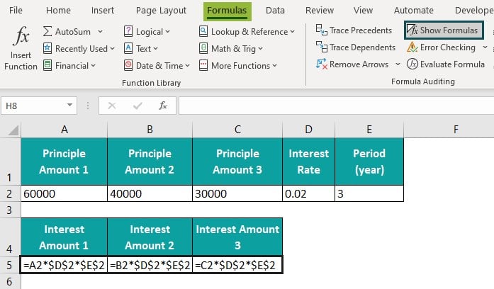
When we click Show Formulas, the formulas in the selected cells are visible, as shown above.
Example #4 – Error Checking (includes Error Checking, Trace Error, and Circular References)
The succeeding example depicts the values, and we will perform calculations and generate #DIV/0! Excel Error. Then, we will perform the Error Checking using the Formula Auditing Tools.
In the table, the data is,
- Column A contains the Value1.
- Column B contains the Value2.
- Column C contains the Output.

The steps for Error checking using the Formula Auditing Tools are as follows:
1: Select cell C2, enter the formula =A2/B2, and press the “Enter” key. The result is a “#DIV/0!” error, as shown below.

2: Next, choose cell C2, i.e., the containing the error – select the “Formulas” tab – go to the “Formula Auditing” group – select the “Error Checking” option, as shown below.

The moment we click Error Checking, the cells containing the formula and the values are shown with the arrows, as shown above.
Example #5 – Evaluate the Formula
Jamie’s company invested in a venture for years on an interest rate of 5%, with a Principal amount. Let us calculate the Simple Interest Amount and Evaluate the Formula using the Formula Auditing Tools.
In the table, the data is,
- Column A contains the Principal Amount.
- Column B contains the Interest Rate.
- Column C contains Time.

The steps to Evaluate the Formula using the Formula Auditing Tools are as follows:
1: Select cell A5, enter the formula =(A2*B2*C2)/100, and press the “Enter” key. The result is ‘$93,714.32’, as shown below.

2: Next, choose cell A5, i.e., the containing the error – select the “Formulas” tab – go to the “Formula Auditing” group – select the “Evaluate Formula” option, as shown below.
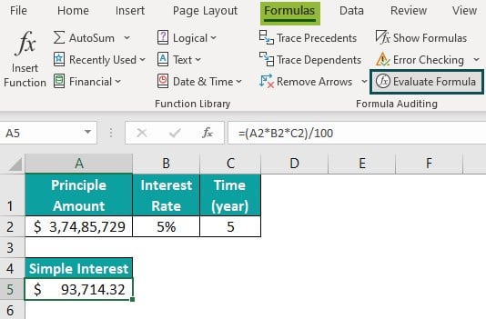
3: The window called the “Evaluate Formula” opens, which shows the Reference cell and the Evaluation section. The Evaluation section displays the formula. To view the step-by-step evaluation of the underlined section of the formula, click “Evaluate”, as shown below.
Here, the first step of the evaluation, underlined, i.e., A2, is calculated.
[Note: The calculation as per the BODMAS technique is followed.]

4: The second step of the evaluation, underlined, i.e., B2, is calculated, and then press the “Evaluate” button to proceed to the next step.

5: Next, the third step of the evaluation underlined, i.e., A2*B2, is calculated, and then press the “Evaluate” button to proceed to the next step.

6: The fourth step of the evaluation, underlined, i.e., C2, is calculated, and then press the “Evaluate” button to proceed to the next step.

7: Later, the fifth step of the evaluation, underlined is calculated, and then press the “Evaluate” button to proceed to the next step.

8: The sixth step of the evaluation, underlined, is calculated, and then press the “Evaluate” button to proceed to the next step.

9: The last step of the evaluation, underlined, is calculated, and then press the “Close” button to close the evaluation of the steps.

Finally, the result we see displayed is the same result of the formula in cell A5, as calculated before, as shown in the above image.
Important Things To Note
- The Formula Auditing tool is under the Formula tab in the separate group.
- The excel keyboard shortcut for the “Show Formula” option is “CTRL + `”, and for the “Evaluate Formula” option is the “F9” key.
- If the cell value is a date, it will be displayed in the number format when we activate the “Show Formulas” command.

Frequently Asked Questions (FAQs)
The Excel Formula Auditing Tools consist of options to troubleshoot the formulas used in a dataset. It ensures that the formulas execute accurately by helping users trace and understand the logic of the formulas used.
The following steps help users to Enable Formula Auditing Tools in Excel.
Step 1: Select the “File” tab – go to the “More…” option from the list – select the “Options” option from the drop-right list, as shown below.
Step 2: The “Excel Options” window appears.
• First, on the left side, select the “Advanced” option from the list.
• Next, on the right side, under r the “Display” section, go to the “Display options for this workbook:” option à select the “Formula Auditing Tools in Excel” option from the drop-down list à select the “All” radio button of the “For objects, show:” section.
• Finally, click “OK”.
We can view the “Formula Auditing Tools in Excel” options, as shown below,
Choose any cell that is a result of a formula – select the “Formulas” tab – go to the “Formula Auditing” group – select any of the required 6 options, as shown below.
Download Template
📥Download the ready-to-use Excel template to practice this tutorial yourself.
Formula-Auditing-Tools-in-ExcelRecommended Articles
This has been a guide to Formula Auditing Tools In Excel. Here we audit formula with tools, Trace-Precedent, Dependent, excel & downloadable excel template. You may learn more from the following articles –

Leave a Reply