
What Is Fractions In Excel?
Fractions in Excel is a number format category that shows the specified value as a fraction instead of its decimal equivalent. The output is a number with a numerator and denominator, separated by a slash sign. To display the fractional values, users can use the inbuilt Fraction format or customize the required formats.
For example, we will display the source data as fractions for the below table that contains a list of numbers.

In column B, we can display the cell values B2:B7 in the fraction form by setting the cells’ format as Fraction in Home → Number Format, and copying the source data in the corresponding target cells.
Use this Fractions In Excel Template to follow along with the examples in this article.
Download Excel Template
When we choose to show Fractions in Excel, the whole part of the decimal number gets displayed as is. And the decimal part, which comes after the decimal point, shows as the fraction, though the original value is still a decimal number.
On the other hand, suppose the given value in a cell is an integer. Then updating the number format of the cell as Fraction will not change the integer format. The output will remain the same, as in the case of row 4.
Key Takeaways
- Fractions in Excel form a number format category that enables one to display a decimal value as a fraction.
- Users can use the Fraction number format to show a fraction in different types, such as up to one, two, and three digits. Excel also offers options to customize the fraction format best suiting the requirements.
- We can apply the Fraction format to cells using the Home → Number Format option or from the Format Cells window.
- We can use the TEXT() to display a fractional value. But we cannot use the value to perform mathematical calculations as the fraction the TEXT function returns will be a text string.
Fractions() Excel Formula
We can insert Fractions in Excel from the Home tab or the Format Cells window, as follows:
#1 – Home Tab
The Fraction number format is available in the Home tab, under the Number Format option.

In this case, we can also use one of the keyboard shortcuts for Fractions in Excel, Alt + H, N, and F.


#2 – Format Cells Window
We can select the Fraction number format category from the Format Cells window that is available in the context menu (which opens by right-clicking the target cell).

The keyboard shortcuts for Fractions in Excel, in this case, are as follows:
- Use the Number dialog box selector in the Home tab to open the Format Cells window, and press N to open the Number tab. And then, click in the Category box and press the F key to select Fraction.

- Click Ctrl + 1 to access the Format Cells window. And then, the rest of the process remains the same as explained above.

How To Use/Write Fractions Excel Function?
We can use the Fractions Excel Function in 2 ways, namely,
- Access from the Excel ribbon.
- Use the Format Cells option.
Method #1 – Access from the Excel Ribbon
Choose the target cell for output à select the “Home” tab → go to the “Number” group → click the “Number Format” option drop-down → select the “Fraction” option, as shown below.

The number format in the chosen cell gets updated as a Fraction.

Method #2 – Use the Format Cells Option
Right-click the required cell to open the context menu → select Format Cells, as depicted below.

The Format Cells window will open, where we can select the required Fraction format from the Fraction category in the Number tab.

Finally, click OK to close the window, and update the cell format as Fraction. Let us take a basic example to learn more.
We will display the given decimal numbers as fractions for the following table with a list of numbers in decimal format, using the Fraction in Excel.

The steps to convert the cell values to fractional values using Fractions in Excel are,
- Select cell range B2:B6, click Home → Number Format option drop-down → Fraction to set the cells’ format as Fraction.

[Alternatively, select cells B2:B6, right-click and select the Format Cells option.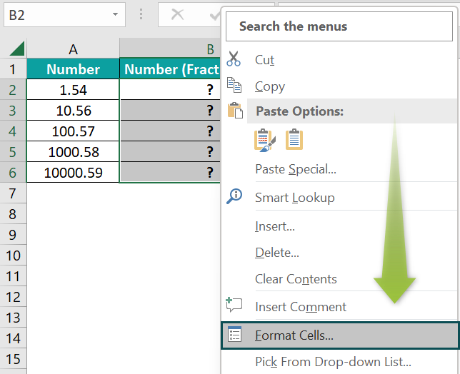
The above step will open the Format Cells window. Here, click the Fraction category in the Number tab. And let us pick the first option as the required Type, which is the default fraction type.
And once we click OK, the window will close with the target cells’ format set as Fraction.] - Select cell B2, enter the formula =A2, and press Enter.
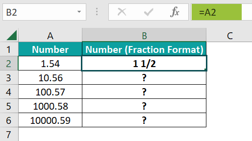
- Using the fill handle, drag the formula to cells B3:B6.
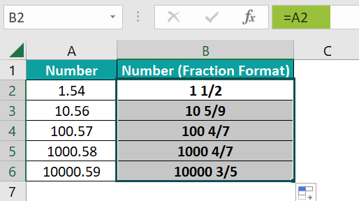
Since the selected fraction type is single-digit, the decimal part in each number gets rounded to the nearest single-digit fraction.
Examples
Let us see a few practical examples of Fraction formats in Excel.
Example #1
We will show the weight values as fractions in tenths format using Excel’s inbuilt Fraction in Excel options.
The below table contains an item list with their weight details in decimals.

The steps to use the inbuilt fraction format option are,
- Step 1: Select cell range C2:C11, right-click to open the context menu, and pick Format Cells to open the Format Cells window.

- Step 2: In the Format Cells window, go to the Number tab and click the Fraction category. And then, in the Type section, scroll down to choose the second last option to get the fractions in tenths format.

Clicking OK will close the Format Cells window, and the selected fraction format will get applied to the chosen cell range.
- Step 3: Select cell C2, enter the formula =B2, and press Enter.

- Step 4: Use the fill handle to enter the formula in cells C3:C11.

The first option under Type, the default fraction format, shows the fraction with a denominator having a single digit. But choosing the second-last option helps display the fraction with the denominator as 10.
Likewise, we can choose the fraction format from the nine options available in the Type section that matches our requirements.
Example #2
At times we might require to display the fractions in a specific format not available in the inbuilt options in the Type section. In such scenarios, we can use customized fraction formats as required.
For example, the below table contains two data sets of decimal values. We will add the two data sets’ values in each row as fractions, with the denominator always being 50. Further, the sum values should also have the same fraction format as the two datasets.

The steps to add Fractions in Excel as per the mentioned requirement are,
- Step 1: Select cell range A2:C6, and click the Number dialog box selector in the Home tab to access the Format Cells window.

- Step 2: In the Format Cells window, select the Custom option as the Category in the Number tab.

And pick the highlighted fraction format as the Type.
- Step 3: Replace the question marks in the denominator in the chosen fraction format with the number 50 to get the required customized fraction type.

Once we click OK, the dialog box will close, and we will see the two data sets’ values as fractions in the desired customized fraction format.

Next, the following steps will add Fractions in Excel cells C2:C6.
- Step 4: Select cell C2, enter the formula =A2+B2, and press Enter.

- Step 5: Implement the formula in the remaining target cells C3:C6 using the fill handle.

The ‘#‘ symbol and the two question marks in the numerator and denominator represent a mixed fraction, with the ‘#’ symbol denoting the integer part. And the remaining section of the format indicates the fractional part.
And replacing the question marks in the denominator with the number 50 ensures the customized fractions display the value 50 in the denominator.
Similarly, we can pick the appropriate fraction format option available in the Custom category and customize the format according to our requirements.
Example #3
We can use the TEXT excel function to display Fractions in Excel.
For example, the table below contains the distance between different destinations as decimals. And we must update the comments in column D stating the distances between the given destinations are the specified miles but in fraction format.

The steps to use the TEXT() and show the miles values as fractions in the comments are:
- Step 1: Select cell D2, enter the below formula, and press Enter.
=”The distance between “&A2&” and “&B2&” is “&TEXT(C2,”# ?/?”)&” miles.”

- Step 2: Apply the formula in cells D3:D6 with the help of the fill handle.

Let us consider the cell D6 expression to check how the formula executes.
The TEXT() returns the specified cell C6 value, 321.9, in the given fraction format. Thus, the function output is 321 8/9.
And the rest of the formula uses the Excel cell references to the two given destinations to display the required comment, with the value of the miles in fraction format.
To suit our needs, we can use a different fraction format in the TEXT().
However, please note that the TEXT() output will be a text string. And hence, we cannot use the resulting fraction for mathematical calculations.
Important Things To Note
- Ensure we apply the fraction format to the target cell and enter the fractional value. Otherwise, Excel will count the value as a date.
- Once a cell has a fraction format, a decimal value or the actual fraction entered in it will display as a fraction.
- When we do not have to perform any calculations on the Fractions in Excel, then, we can set the specific cell format as Text in the Home → Number Format and type the fraction. It will ensure the entered fractional value is not reduced or converted into decimal.
Frequently Asked Questions (FAQs)
We can multiply fractional values with whole numbers in Excel using the following steps. Let us see them with an example.
The following table shows two value sets. While the first set contains whole numbers, the second set shows decimals. We must display the decimals as fractional values, then multiply the fractions with the whole numbers in each row and show the products in column D.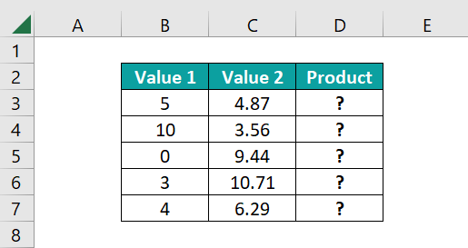
The steps to multiply fractional values with whole numbers are as follows:
• Step 1: Select the cell range C3:C7, and go to Home → Number Format drop-down → Fraction to set the cell range format as Fraction.
• Step 2: Select cell D3, enter the formula =B3*C3, and press Enter.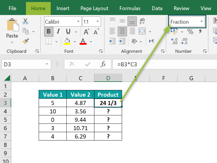
Once we multiply the fractional value with the whole number in the target cell, the cell format will automatically get updated as a Fraction with the product displayed as a fraction.
• Step 3: Copy the formula in the remaining target cells D4:D7 with the help of the fill handle.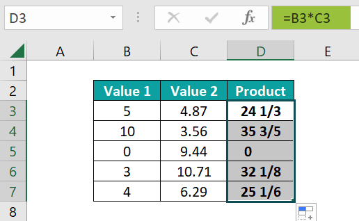
We can copy and paste Fractions in Excel using the following steps:
1) First, ensure the fractions are in the required format.
2) Then select the cell range containing the fractional values and press Ctrl + C.
3) Finally, choose the first target cell, where we must paste the fractions in one cell after the other, and then press Ctrl + V.
The above steps will copy and paste the values in the target cells as fractions.
We can convert fractions to decimals in Excel using the below steps:
1) First, select the cell range containing the fractional values.
2) Next, navigate the path Home → Number Format drop-down → General to change the cell range format from Fraction to General.
Once we set the cell range format as General, the fractions will get displayed as decimal values inside the cells and in the Formula Bar.
Use this Fractions In Excel Template to follow along with the examples in this article.
Download Excel TemplateRecommended Articles
Continue with these related resources when you want the next practical step in this topic.
- Mathematical Functions in Excel
- Excel Minus Formula
- Excel Subtraction Formula
- Multiply Formula In Excel
- Divide In Excel
Explore the full Excel Math Functions guide or browse Excel Resources.