
What is Ratio in Excel?
In Mathematics, generally, the ratio is defined as the comparison of two or more quantities of the same kind with respect to each other. It indicates how many times one value is in comparison to another value. The definition of ratio holds the same for Excel, too. However, Excel has no built-in function to calculate the ratio directly. But many methods help you calculate and display the ratio. For instance, the ages of John and his uncle are 15 and 45, respectively. To find the ratio of their ages, we can apply the following formula in cell C2:
=(A2/B2)&” : “&1. Here, we divide cell A2 by B2 and with the ampersand (&) symbol, we put the ratio sign(:). By doing this, we divide one value by another and compare it against one.

Use this Ratio in Excel Template to follow along with the examples in this article.
Download Excel TemplateKey Takeaways
- The ratio in Excel compares two numbers with respect to each other. There is no fixed method to find the ratio in Excel. You can find the ratio using functions like GCD, ROUND, SUBSTITUTE, and text.
- The & symbol is used to concatenate various parts of the formula. Using the ROUND function, you can specify the number of decimal places of any number occurring in the ratio.
- When one of the numbers is non-numeric, you get the #VALUE! Error when using any of the above formulas.
Ratio Excel Formula
There’s no exclusive function for finding the ratio in Excel. However, we can use several simple formulas to find the ratio. One such simple method is the simple Division method.
The formula to find the ratio of two numbers using the division method is:
= Value1/ Value2 &” : “&“1”
Here,
- Value1 and Value2 are the two numbers whose ratios we want to find
- “:” is the symbol for the ratio
- “&” is used to append the ratio symbol “:” to the two numbers
- 1 is the value with which the two numbers are compared
Another simple division formula used to find the ratio is:
=Value1/Value2&” : “&Value2/Value2
- Value1 and Value2 are the two numbers whose ratios we must find
How to Calculate Ratio in Excel?
Four methods can calculate the ratio in Excel.
- The simple division method
- Using the GCD method
- With the ROUND() function
- Using SUBSTITUTE and TEXT function
We can enter these formulas manually in the Excel cells. Here’s an example of entering the formula by the division method to find the ratio of two numbers.
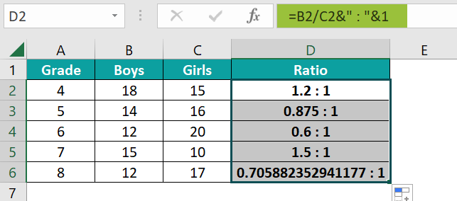
Let us take the example of two columns that contain the number of boys and girls in different grades in a school. But first, let us calculate each class’s ratio of boys and girls.

We can calculate Ratio in excel using the steps below –
- Now, let us apply a simple division formula to find boys to girls’ quick ratio in Excel. Apply the formula =B2/C2&” : “&1 in cell D2 and press Enter.
Here,
• ‘&’ is used to concatenate the different parts of the formula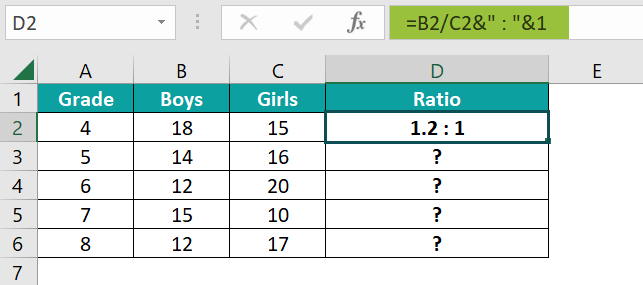
- As observed, the boys-to-girls ratio is given as 1.2: 1. Now, apply the formula to the rest of the cells from D3 to D6 by dragging the Autofill handle. You get the ratio of boys to girls for each grade.
Applying the GCD Function to Find the Ratio
Another way of calculating the ratio is using the GCD function from the Excel ribbon in a formula. But you may only sometimes require the ratio denominated by 1. Sometimes, it can be expressed in the form of their divisors. In such cases, you can use the GCD to find the ratio of two numbers.
Let us take an example of the width and height of a structure. Here, we must find the ratio. Let us look at how to do it with GCD in Excel.

- Step 1: We use GCD or the greatest common divisor to find a common denominator for both numbers. Enter the formula =GCD(A2,B2) in cell C2. Press Enter.

- Step 2: Drag the Autofill handle until C8 to get the GCD for the other numbers.

- Step 3: Now, enter the formula =A2/C2 & “:” & B2/C2 in cell C2.
Here, we are finding the GCD of the two numbers, which makes up for the terms of the ratio. Press Enter. You get the ratio of the width ratio to the height as 4: 5.

- Step 4: Drag the Autofill handle from D2 to D8 to get the ratios for all the other numbers.

Thus, we can easily calculate and simplify ratio in Excel even without the availability of a direct function.
Examples
In the previous section, we have seen how to find and show ratio in Excel. Now, let us look at another simple division method to find the ratio of two numbers.
Example #1
We have an example where, to prepare hot chocolate for a group, a chef experiments with different amounts of milk and chocolate to arrive at the right recipe; each time, he notes down the quantity which satisfies his customers. Find the ratio of the milk to the chocolate he uses each time.

- Step 1: Enter the details of the milk and chocolate used in Columns A and B, respectively. Now, let us apply the formula =Value1/Value2&”: “&Value2/Value2 to find the ratio of the milk to chocolate.
Type =A2/B2&” : “&B2/B2 in C2 and press Enter.

- Step 2: Now, drag the handle up to cell C6. You get the various ratios. This formula is just another version of = Value1/ Value2 &” : “&“1”.

Hence, the chef settles for the ratio of 6.25:1 for milk: chocolate, as the customers prefer it the most.
Example #2
Only at times, we get such rounded ratios. Mostly, we get ratios like 1:6.7777777777 in Excel. One way to round up these values is through the ROUND Excel function. The ROUND function rounds the values to the number of digits mentioned.
Let us look at an interesting example of using the ROUND function.
We have the diameter of the Sun in cell B1. Let us compare the diameters of all the other planets to see how big they are with respect to the Sun.

- Step 1: Enter the formula =ROUND($B$2/B3,1)&”:”&1 in cell C2. Press Enter.
- ROUND helps you get the value up to any desired decimal place.
- We can’t adjust the result by applying the Number format or using the Decrease Decimal feature since only a part of the ratio is a decimal value.
- The rest of the values are considered text and can’t be treated as a number. It is where the ROUND formula comes in handy.
- ROUND() returns the quotient to a single decimal place after the division.
- We have fixed the cell reference in Excel for the diameter of the sun since it will be used repeatedly.

- Step 2: You can observe that the ratio of the Sun to Mercury is 288.3:1, which means that the Sun is approximately 288 times larger than Mercury.
Drag the Autofill handle to C10 to get the rounded ratios for all the other planets.

Therefore, we get the size comparison of all planets with respect to the Sun. Interestingly, the Earth is 109 times smaller than the Sun!
Example #3
Now, let us look at another example of finding the ratio using the SUBSTITUTE function1 and TEXT excel functions. Below is a list of students who passed or failed in Maths in different grades. Again, we can use the SUBSTITUTE function, which replaces one text with another, while the TEXT function provides the text in a particular format.

- Step 1: Use the formula =SUBSTITUTE(TEXT(C3:D3,”#/######”),”/”,”:”) and press Enter.
- Here, using the TEXT function, the numbers 16 and 7 are converted to a fraction.
- Now, the output of the TEXT function is 16/7.
- Next, the SUBSTITUTE function can format ratio in Excel and converts the number with the / “slash” to a ratio by replacing the “/” with “:”

- Step 2: Now, drag the Autofill excel handle from E3 to E7 to get the ratios of students who have passed to those who have failed.

Thus, we can get the ratio in different Excel formats, including the GCD function, the division method, and the SUBSTITUTE function.
Important Things to Note
- Excel has no specific functions to find ratios, but functions like the GCD function help quickly determine the ratio.
- You can use the ROUND function to round the values to the nearest decimal when one of the numbers in the ratio is a decimal.
- The ratio of two numbers can be found even using the CONCATENATE Excel function instead of the & symbol.
Frequently Asked Questions (FAQs)
There is no direct function to find the ratio in Excel. You have four different ways to find it. They are:
• The division method
• Using the GCD function
• With the ROUND function
• Using the SUBSTITUTE and TEXT function
There is no specific function in Excel to calculate the loss ratio. It is the losses incurred by brokers, insurers, etc., in benefits and claims. It can be calculated in Excel with the following formula.
Loss Ratio = (Losses Due to Claims + Adjustment Expenses) / Total Premium Earned
An odds ratio shows the probability of an event happening to that of the non-occurrence of the event. For example, suppose there is a dice. The odds ratio gives the odds of throwing a three.
(Probability a three is thrown (1/6))/(Probability of a three not thrown (5/6))
The current ratio compares a firm’s current assets to its current liabilities. You can calculate the sum of all existing assets and liabilities in Excel and find its ratio.
Use this Ratio in Excel Template to follow along with the examples in this article.
Download Excel TemplateRecommended Articles
Continue with these related resources when you want the next practical step in this topic.
- Mathematical Functions in Excel
- Excel Minus Formula
- Excel Subtraction Formula
- Multiply Formula In Excel
- Divide In Excel
Explore the full Excel Math Functions guide or browse Excel Resources.