
What Is Highlight Duplicates In Google Sheets?
Highlight duplicates in Google sheets, as the name suggests, highlights the duplicate values from the given data set in Google sheets. This option helps users identify or find the repetitive value.
We generally use Conditional Formatting option to highlight duplicates in Excel and the same rule goes for google sheets also.
Use this Highlight Duplicates In Google Sheets Template to follow along with the examples in this article.
Download Excel TemplateFor example, consider the below table showing names of various students in a class in the cell range A1:A9.

Now, let us highlight the duplicate values using conditional formatting.
The steps are:
Step 1: To begin with, select the range where we have to find or highlight duplicates. In this example, it is the cell range A1:A9.
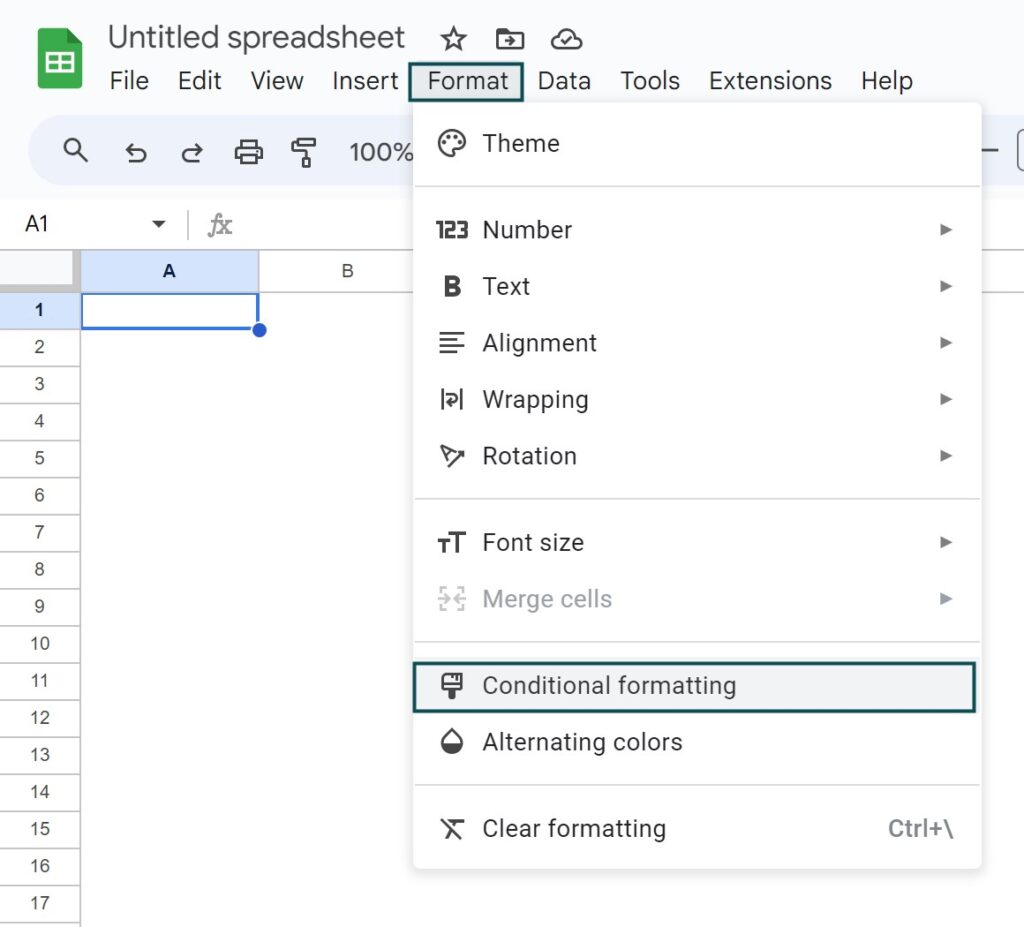
Step 2: Next, click on Format tab and select Conditional Formatting.
Step 3: Now, the Conditional Format rules tab appears on the right side.
Then, select the Single Color and fill in the Apply to range, Format rules and Formatting style.
Step 3: Finally, press Done option.
Now, we can see highlighted duplicates.

Likewise, we can highlight duplicates.
In this article, let us learn how to highlight duplicates and how to use the Conditional Format Rules tab.
Key Takeaways
- Highlight duplicates in google sheets helps users find the duplicate or repetitive values in the given data set.
- This function is highly useful while dealing with large data sets as manually identifying or highlighting duplicating values is close to impossible.
- We can highlight duplicates using conditional formatting option in google sheets.
- Using conditional formatting, we can highlight cells, rows or columns in google sheets with just a click.
- Remember, instead of conditional formatting, we can also use add-on to highlight duplicates in google sheets.
How To Highlight Duplicates In Google Sheets?
We can highlight duplicates in Google sheets with the following steps. They are:
Step 1: Select the range and click on the Format tab.

Step 2: Then, click on Conditional Formatting under the Format tab in Google Sheets.
Step 3: The Conditional Format rules tab appears on the right side.

Step 4: Now, click on Single Color option.
Step 5: In the Apply to range option, select the cell range within which we want to highlight the duplicates.
Step 6: Then, under the Format Rules option, click on the drop down and scroll down to select Custom Formula is

Step 7: Now, the Value or Formula bar appears. Meanwhile, insert the COUNTIF function.
Then, select the desired cell range.
Step 8: Finally, click on Done.
Now, we can find the duplicates values immediately.
Let us learn how to highlight duplicates with detailed examples.
Examples
Example #1
Consider the below table showing subject list in google sheets.

Now, let us learn how to highlight duplicates.
The steps are:
Step 1: To start with, select the range A2:A8 and then, click on the Format tab.
Step 2: Next, click on Conditional Formatting under the Format tab in Google Sheets.

Step 3: Now, the Conditional Format rules tab appears on the right side.

Step 4: Next, click on Single Color option.
Step 5: Now, in the Apply to range option, select the cell range within which we want to highlight the duplicates.

Step 6: Then, under the Format Rules option, click on the drop down and scroll down to select Custom Formula is

Step 7: Now, the Value or Formula bar appears.
Next, insert the COUNTIF function =COUNTIF($A$2:$A$8,$A2)>1

Step 8: Finally, click on Done.
We can find the duplicates values immediately.

Likewise, we can highlight duplicates.
Example #2
In this example, let us learn how to highlight duplicates in google sheets in multiple columns.
Consider the below table showing names, education and profession in columns A, B and C respectively.

Now, let us learn how to highlight duplicates.
The steps are:
Step 1: To begin with, select the range A2:C9 and then, click on the Format tab.
Step 2: Then, click on Conditional Formatting under the Format tab in Google Sheets.

Step 3: Now, the Conditional Format rules tab appears on the right side.

Step 4: Now, click on Single Color option.
Step 5: Next, in the Apply to range option, select the cell range within which we want to highlight the duplicates.

Step 6: Then, under the Format Rules option, click on the drop down and scroll down to select Custom Formula is
Step 7: Now, the Value or Formula bar appears.
Next, remember to insert the COUNTIF function =COUNTIF($A$2:$C$9,$A2)>1
Step 8: Finally, click on Done.
We can find the duplicates values immediately.

Likewise, we can highlight duplicates.
Example #3
Consider the below table showing fruits and colors in cell range A1:B7.

Now, let us learn how to highlight duplicates in google sheets with the following steps.
The steps are:
Step 1: To begin with, select the range A2:B7 and then, click on the Format tab.
Step 2: Next, click on Conditional Formatting under the Format tab in Google Sheets.

Step 3: Now, the Conditional Format rules tab appears on the right side.

Step 4: Now, click on Single Color option.
Step 5: Next, in the Apply to range option, select the cell range within which we want to highlight the duplicates.

Step 6: Then, under the Format Rules option, click on the drop-down and scroll down to select Custom Formula is
Step 7: Now, the Value or Formula bar appears.
Remember, we need to insert the COUNTIF function.
Step 8: Finally, click on Done.
Now, we can find the duplicates values immediately.

Likewise, we can highlight duplicates.
The Cautions Governing Duplicate Values
We need to make sure the following points while using conditional formatting to highlight supplicates in google sheets.
- To start with, we need to make sure there are no other conditional formatting rules given in the table.
- Next, the data should be error free and should be free from empty spaces to make sure the duplicates are highlighted.
- Remember not to select headers while choosing cell range to highlight duplicates.
Important Things To Note
- Google sheets highlight duplicates function finds the repetitive values in the data.
- To highlight duplicates in google sheets, click on Format > Conditional Formatting and then, click on Single Color option.
- Then, we need to choose the desired cell range and click on the formatting options, formula and color in the same tab.
- We can highlight duplicates in google sheets for any number of columns, and rows.
Frequently Asked Questions (FAQs)
Now, consider the below table showing names of various students in a class in the cell range A1:A6.
Now, let us highlight the duplicate values using conditional formatting in Google sheets.
The steps are:
Step 1: To start with, select the range where we have to find or highlight duplicates. In this example, it is the cell range A1:A6.
Step 2: Next, click on Format tab and select Conditional Formatting.
Step 3: Now, the Conditional Format rules tab appears on the right side.
Then, select the Single Color and fill in the Apply to range, Format rules and Formatting style.
Step 3: Finally, press Done option.
Now, we can see highlighted duplicates in Google sheets.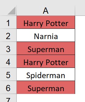
Likewise, we can highlight duplicates.
We need to remember the following points while using highlight duplicates in Google sheets:
• First, make sure there are no spelling mistakes in the data to avoid errors
• Next, ensure there are no empty spaces
• Similarly, select the cell range properly
Remember, we can simply select Format > Conditional Formatting > and delete the conditional formatting rule to delete or remove highlight duplicates in Google sheets.
Use this Highlight Duplicates In Google Sheets Template to follow along with the examples in this article.
Download Excel TemplateRecommended Articles
Continue with these related resources when you want the next practical step in this topic.
- Data Validation In Google Sheets
- Format Cells in Google Sheets
- Conditional Formatting In Google Sheets
- Filter Function In Google Sheets
- SORT in Google Sheets
Explore the full Google Sheets Data Cleaning Validation and Formatting guide or browse Google Sheets Resources.