IFNA Excel Function

What Is IFNA Function In Excel?

The IFNA function in Excel is an inbuilt Logical function. It returns the specified value if the given formula’s output is the #N/A error. Else, the IFNA Excel function output is the formula’s return value. Therefore, users can use the IFNA() to capture the #N/A errors and display a customized message in place of them.

For example, the following table contains a list of error values.

Suppose we must check the error values for the #N/A error and show the result as Yes if the specific cell contains the #N/A error and the cell value otherwise. And assume the column B cell range B2:B8 are the target cells. Then, applying the IFNA Excel function in the target cells can fetch us the required result.

The IFNA() accepts the source data cell as the first argument, and the second argument shows the message we must display instead of the #N/A error. Cell A3 is the only cell in the range A2:A8 that contains the #N/A error. And hence, the target cell B3 formula returns Yes as the output.

What Is IFNA Function In Excel?

The IFNA Excel function checks if a value or a formula has the #N/A error. If the condition holds, the IFNA() returns the value we specify. Otherwise, it returns the value or the formula’s output it verified for the #N/A error.
The IFNA function helps trap the #N/A error when working with massive data sets and allows users to display a customized message instead of the error value.
As inputs, the IFNA function accepts two mandatory arguments, value and value_if_na.
The IFNA function works well with the value argument being expressions such as the VLOOKUP() and the INDEX-MATCH formula.

IFNA() Excel Formula

The IFNA Excel function syntax is:

where,

value: The value or expression to check for the #N/A error.
value_if_na: The value the IFNA Excel function should return if the given value or the expression result is the #N/A error.

Both the arguments in the IFNA() are mandatory.

Excel VBA – All in One Courses Bundle (35+ Hours of Video Tutorials)

If you want to learn Excel and VBA professionally, then Excel VBA All in One Courses Bundle (35+ hours) is the perfect solution. Whether you’re a beginner or an experienced user, this bundle covers it all – from Basic Excel to Advanced Excel, Macros, Power Query, and VBA.

Start Learning Now

How To Use IFNA Excel Function?

The steps to use the IFNA Excel function are as follows:

First, ensure the given value or the formula is accurate.
Then, choose the required target cell and enter the IFNA().
Finally, press Enter to view the IFNA function return value.

Here is an example to explain the above steps in detail. The table below shows a list of numbers.

How to use IFNA Excel Function - Basic Example

Suppose the requirement is to determine if the given numbers are multiples of 2 and display the output in column B. Then, here is how we can apply the IFNA() in the target cells and get the required data.

To begin with, select the target cell B2, enter the below formula, and then, press Enter.
=IFNA(IF(MOD(A2,2)=0,”Number is a multiple of 2.”,#N/A),”Number is not a multiple of 2.”)

We can also select the target cell and go to Formulas → Logical → IFNA to apply the function using the Function Arguments window.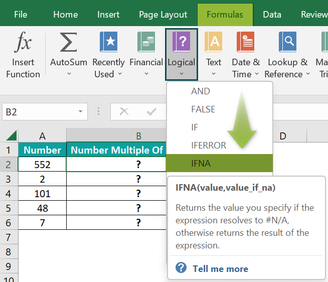

Next, we must enter the values in the two fields in the Function Arguments window.

Finally, clicking OK will execute the IFNA() in the target cell.
Next, apply the above formula in cell range B3:B6 using the fill handle.

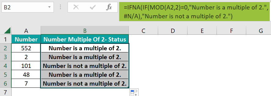
Let us consider the cell B6 expression to check how the formula works. The IF() is the value argument. So, first, the MOD() finds 7 mod 2 to return 1, which is not equal to 0. Thus, the IF() condition is FALSE, and the function returns the FALSE value, #N/A.

Finally, the IFNA() checks the IF() return value for the #N/A error. And as the IF() output is the required error value, the IFNA() returns the message “Number is not a multiple of 2”, as the status.

Examples

Check out the following examples to apply the IFNA Excel function in the best way possible.

Example #1

Here is an example of the IFNA with the VLOOKUP excel function as the value argument.

The first table shows a team’s appraisal details.

Suppose the second table contains employee names, and you need to update their appraisal status in cell range B15:B16 based on the first table. Then, here is how we can apply the IFNA Excel function in the target cells and get the status data.

Step 1: First, select the target cell B15, enter the below formula, and press Enter.

=IFNA(VLOOKUP(A15,$A$2:$B$11,2,0),”Appraisal Pending”)

Step 2: Next, drag the Excel fill handle down, and enter the formula in cell B16.

The VLOOKUP() looks up the employee name specified in the second table in the first table. It returns the corresponding appraisal status for the given employee name from the first table. Else, it returns the #N/A error.

In the case of the cell B15 formula, the VLOOKUP() returns Gretchen Hines’s appraisal status, Complete, as the name is present in the first table. And thus, the IFNA() result is the VLOOKUP() return value, Complete.

On the other hand, the cell A16 value, Kevin Reed, is not present in the first table. So, the VLOOKUP() output is the #N/A error. And the IFNA() displays the message “Appraisal Pending” as a replacement for the error value.

Example #2

This illustration shows how the IFNA Excel function works when the value argument is a formula containing the INDEX and MATCH Excel functions.

The first table shows an items list with their weight details.

And assume we need to determine the weight for the item specified in cell E2 of the second table based on the first table data and display the result in cell F2.

Then, we can apply the IFNA Excel function in the target cell to get the required data.

Step 1: To start with, select the target cell F2, enter the below formula, and then, press Enter.

=IFNA(INDEX(B2:B11,MATCH(E2,A2:A11,0)),”Data Not Available”)

First, the MATCH() checks for the cell E2 value, item_15, in the cell range A2:A11. As the required item is not present in the specified cell range, the function returns the #N/A error. And thus, the INDEX Excel function also returns the #N/A error as the value the #N/A is not present in the cell range B2:B11 to return the cell reference or value at the row-column intersection.

Finally, as the given formula (value argument) output is the #N/A error, the IFNA() returns the message “Data Not Available” to display instead of the error value.

Example #3

This example explains using the IFNA Excel function as an array formula in Excel.

The first table shows a list of students and their score details.

Consider the second table contains some students’ names, and we must get their scores in cell range F2:F5 based on the first table data. Then, we can execute the IFNA Excel function as an array formula in the target cells and achieve the required data.

Step 1: First, select the cell range F2:F5 and then, enter the below formula.

=IFNA(VLOOKUP(E2:E5,A2:B11,2,0),”Data Not Found”)

Step 2: Next, press the Ctrl + Shift + Enter keys to execute the above expression as an array formula.

{=IFNA(VLOOKUP(E2:E5,A2:B11,2,0),”Data Not Found”)}

The VLOOKUP() looks up the cell range E2:E5 values in the first table to return each student’s score based on the first table. As it finds the cells E2 and E4 values in the first table, it returns their respective scores, 87 and 77. And as the function does not find the cell E3 and E5 names in the first table, it returns the #N/A error.

And, based on the VLOOKUP() outputs, the IFNA() returns the message “Data Not Found” if the VLOOKUP() output is the #N/A error. Otherwise, its output is the looked-up score the VLOOKUP() returns.

Important Things To Note

The IFNA function works only for the #N/A error in a spreadsheet.
For the value or value_if_na argument supplied as an empty cell, the IFNA Excel function considers it as an empty string (“”).
Suppose the value argument is an array formula. Then the IFNA function output is an array of return values for the cell range specified in the value argument.

Frequently Asked Questions (FAQs)

1. Where is the IFNA function in Excel?

The IFNA function in Excel is in the Formulas tab. Navigate the path Formulas → Logical → IFNA to access and apply the function in the required target cell.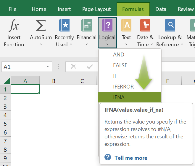

2. How to apply IFNA function in Excel VBA?

We can apply IFNA function in Excel VBA using the method mentioned below:

Application.Worksheetfunction.IfNa(value,value_if_na)

In the above method, the arguments, value, and value_if_na have the same meaning defined in the IFNA() Excel Formula section.

The example below shows how to apply the abovementioned method in Excel VBA.
The following table contains a list of values.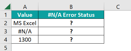

Suppose the requirement is to determine if the given value is the #N/A error, display the status in column B, and the given data otherwise. Then, here is how we can apply the IFNA function in Excel VBA using the method mentioned above.

• Step 1: With the current sheet containing the above table open, press the Alt + F11 keys to open the VBA Editor.

• Step 2: Choose the required VBAProject, click Insert, and then Module to open a new module window, Module1.

• Step 3: Enter the code to apply the IFNA function in the target cells.

Sub IFNA_fn()

Dim Ws As Worksheet
Set Ws = worksheets(“FAQ_2”)

Ws.Range(“B2”) = Application.WorksheetFunction.IfNa(Ws.Range(“A2”), “The value is #N/A error.”)
Ws.Range(“B3”) = Application.WorksheetFunction.IfNa(Ws.Range(“A3”), “The value is #N/A error.”)
Ws.Range(“B4”) = Application.WorksheetFunction.IfNa(Ws.Range(“A4”), “The value is #N/A error.”)

End Sub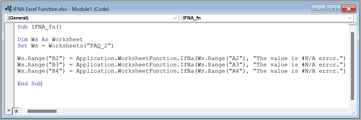

• Step 4: Using the Run Sub/UserForm option, execute the code.

• Step 5: Go to the active worksheet to view the required result.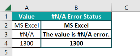

The method checks the value in the specified cell reference. And if the data is the #N/A error, as in cell A3, the function returns the value, “The value is #N/A error”, in the corresponding target cell B3. Otherwise, the IFNA() output is the given value, as in the target cells B2 and B4.

3. What is the difference between the IFNA and IFERROR functions?

The difference between the IFNA and IFERROR functions is that the IFNA() traps only the #N/A error. On the other hand, the IFERROR() identifies the different Excel errors, such as the #N/A, #DIV/0, #NAME, #NUM, #VALUE, and #REF.

The IFNA() best suits the LOOKUP functions, as these functions ideally return the #N/A error if they do not find the lookup value. And the IFERROR() is useful when the calculations involve complex formulas containing Excel functions returning different error values.

Download Template

This article must be helpful to understand the IFNA Excel Function, with its formula and examples. You can download the template here to use it instantly.

IFNA Excel Function Download

IFNA Excel Function