
What Is Percentage In Excel?
Percentage in Excel is a number format category that displays a numeric value as a fraction of 100 followed by the percentage symbol ‘%’.
Users can use the Percentage option to represent fractions conveniently and perform complex mathematical calculations involving percentages.
Use this Percentage In Excel Template to follow along with the examples in this article.
Download Excel TemplateFor example, the below table shows income, expenses, and savings data.
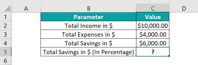
We can display the total savings of the total income in the percentage format by setting the Number Format in the Home tab as Percentage.
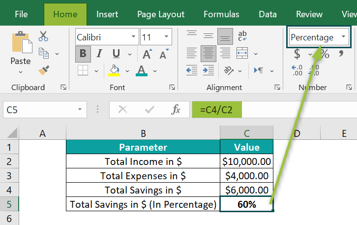
Thus, we can set the specified cell value, if it is a number or the formula in the target cell returns a valid number, to the Percentage format.
Key Takeaways
- The Percentage in Excel is a Number Format type, which displays a number as a proportion of 100, followed by the ‘%’ symbol.
- Users can use the Percentage format to display fractional values more straightforwardly. And the option is useful when the mathematical calculations involve percentage values.
- We can access the Percentage format from the Home tab, or the Format Cells window. Also, we can set the required custom Percentage format from the Format Cells window.
- The keyboard shortcut Ctrl + Shift + % enables one to set the data format in the chosen cell as Percentage.
Percentage Excel Formula
There is no inbuilt Excel formula, as the Percentage is not a function or a mathematical expression, instead, it is a format.
We can use the following ways to change the numeric cell value or the result of a formula to the Percentage format, namely:
- Home tab and the excel keyboard shortcut Alt + H, N, and P.
- Home tab – Percent Style icon or its keyboard shortcut Alt + H and P or Ctrl + Shift + %.
- Format Cells window.
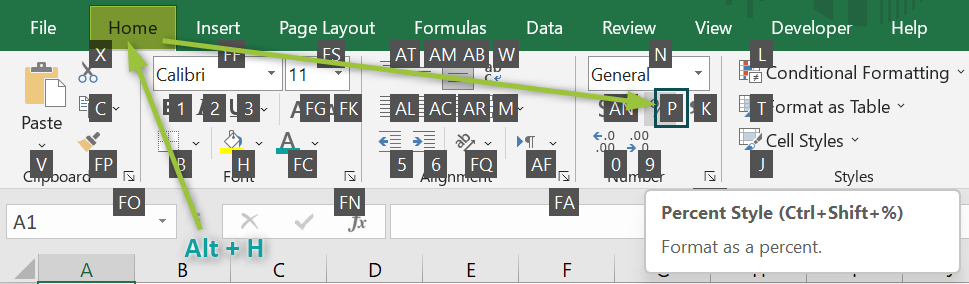
#1 – Home tab or the keyboard shortcut Alt + H, N, and P
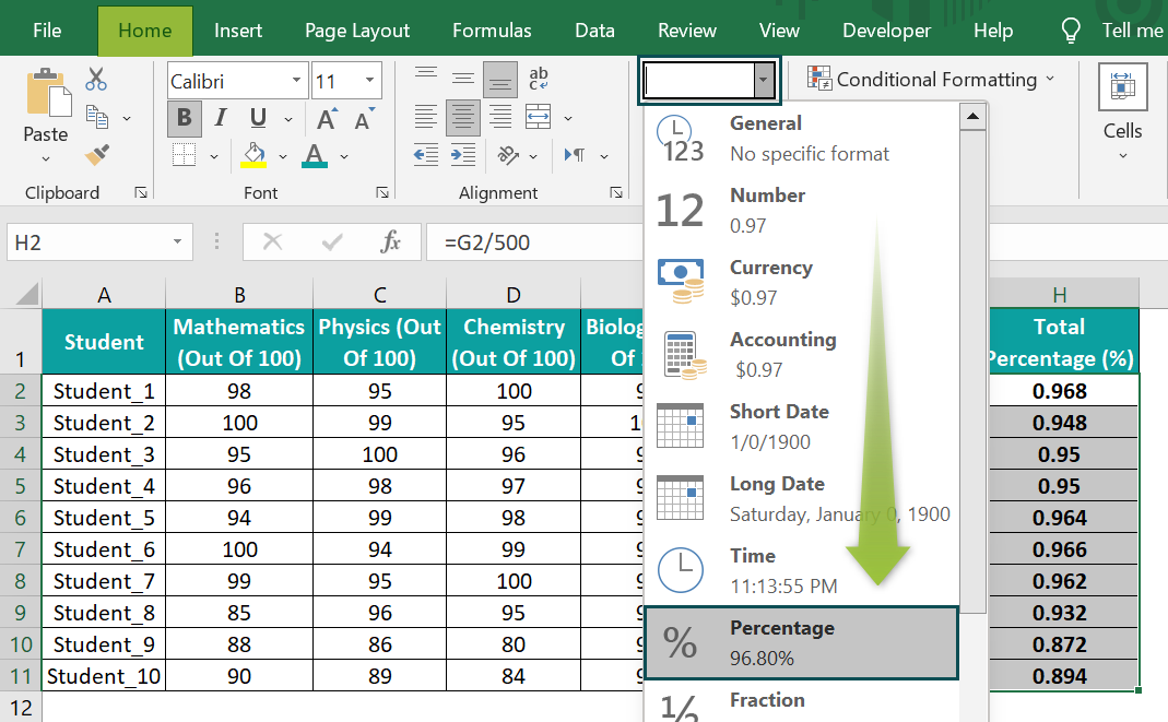
The Percentage in Excel is available in the “Home” tab → “Number” group → “Number Format” option drop-down → “Percentage” option, as shown below.

We can also apply the keyboard shortcut Alt + H, N, and P to use the above option and find a Percentage in Excel.

#2 – Home tab – Percent Style icon or its keyboard shortcut Alt + H and P or Ctrl + Shift + %
We can use the Percent Style icon in the “Home” tab → “Number” group → “Percent Style” option, as shown below.
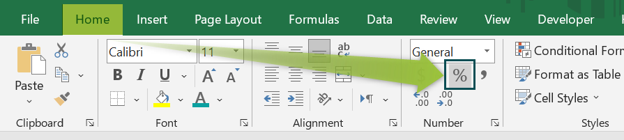
And the keyboard shortcuts to access this option are Alt + H and P or Ctrl + Shift + %.
#3 – Format Cells
We can pick the Percentage number format category from the Format Cells window.
The Format Cells is an option in the context menu (which opens when we right-click the chosen cell or any cell).

The keyboard shortcuts, in this case, are as follows:
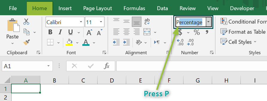
- Use the Number dialog box selector in the Home tab to open the Format Cells window, and press N to open the Number tab. And then, click in the Category box, and press the P key to select Percentage.
- Click Ctrl + 1 to access the Format Cells window. And then, the remaining process is the same as explained above.

How To Calculate Percentage In Excel?
We can calculate the percentage value in Excel in 2 ways, namely,
- Access from the Excel ribbon.
- Use the Format Cells option.
Method #1 – Access from the Excel ribbon
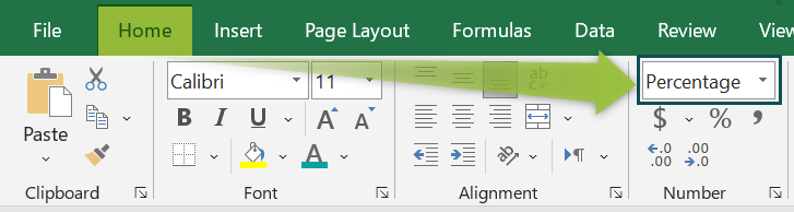
Choose a target cell for output → select the Home tab → click the Number Format option drop-down → select the Percentage option, as depicted below.
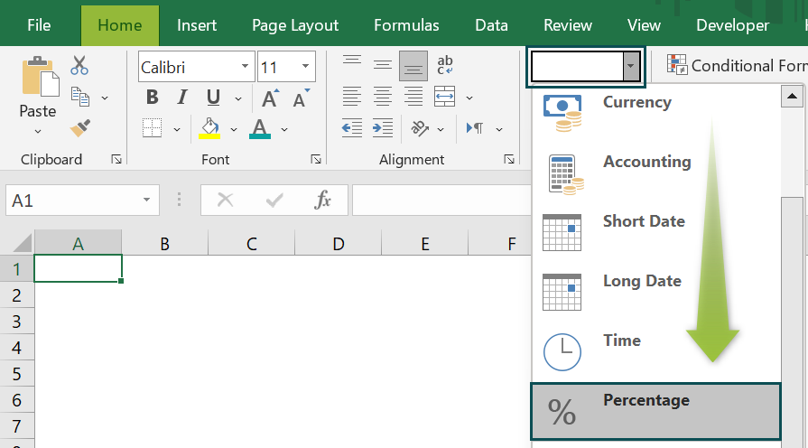
The number format in the target cell gets updated as Percentage.
Method #2 – Use the Format Cells option
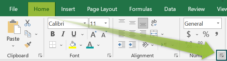
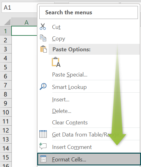
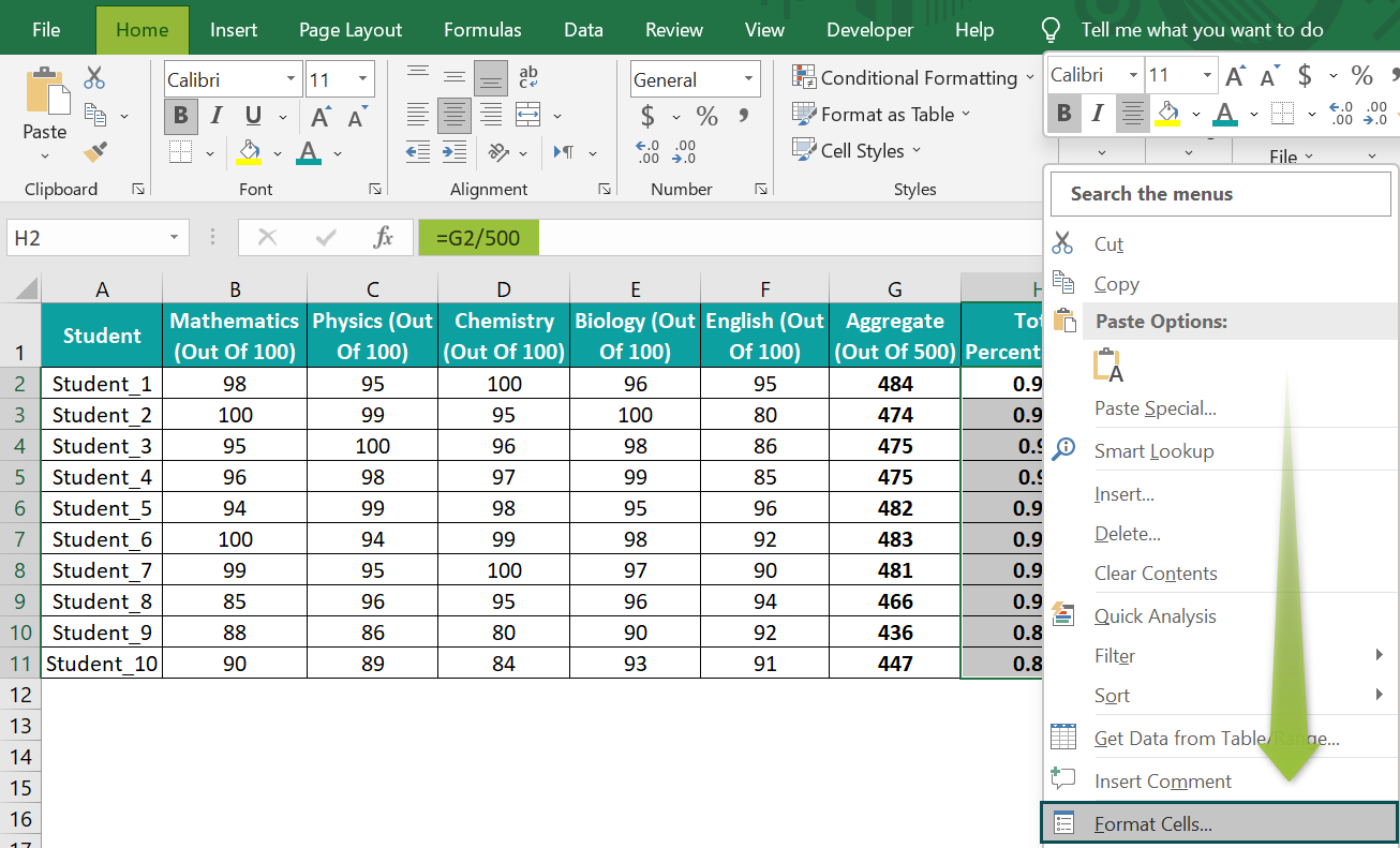
Right-click the target cell to open the context menu → select Format Cells, as shown below.
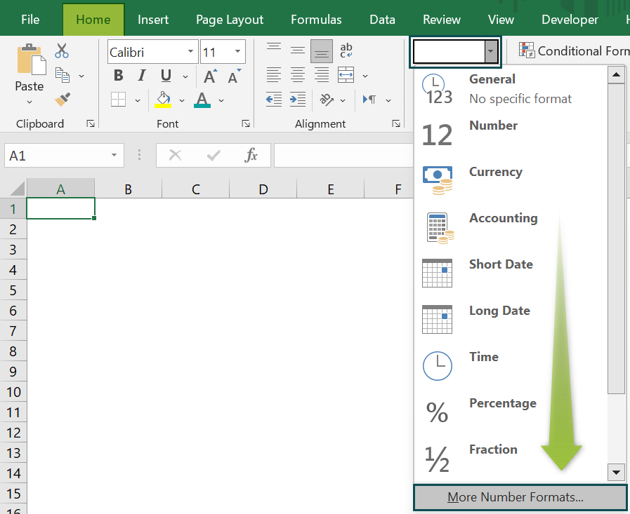
Alternatively, navigate the path Home → Number Format → More Number Formats to open the Format Cells window.
We can now access the Format Cells window, where we can set the required Percentage number format (Decimal places) from the Percentage category in the Number tab.
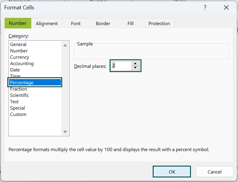
And clicking OK (highlighted in the above image) will close the dialog box and update the cell format as Percentage.
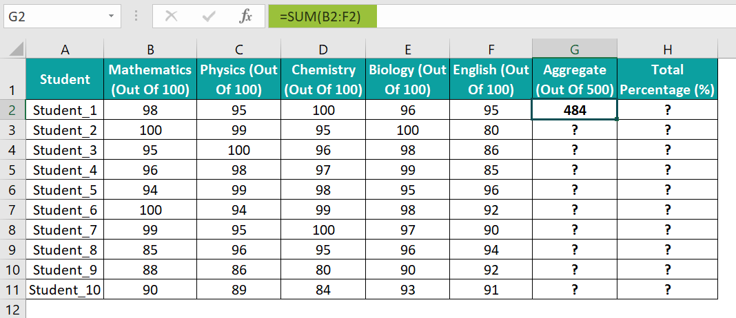
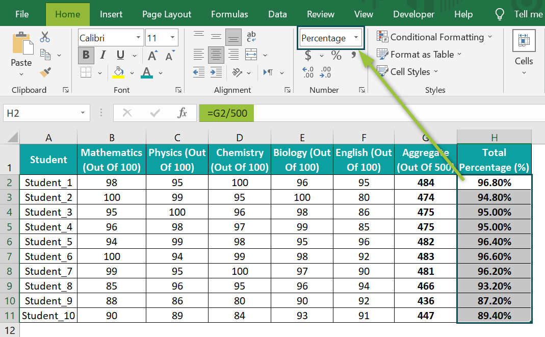
The below table contains the scores of ten students in a class in five subjects. We will determine the aggregate of all subjects and the total percentage, up to two decimal places, secured by each student.
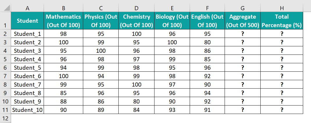
The steps to perform the required calculations and get the results in percentage format are,
- Select the target cell G2, enter the formula =SUM(B2:F2), and press Enter.

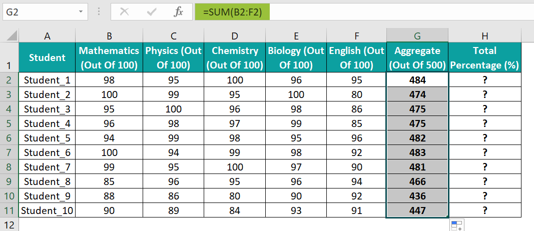
- Using the fill handle, drag the formula from G2 to G11.

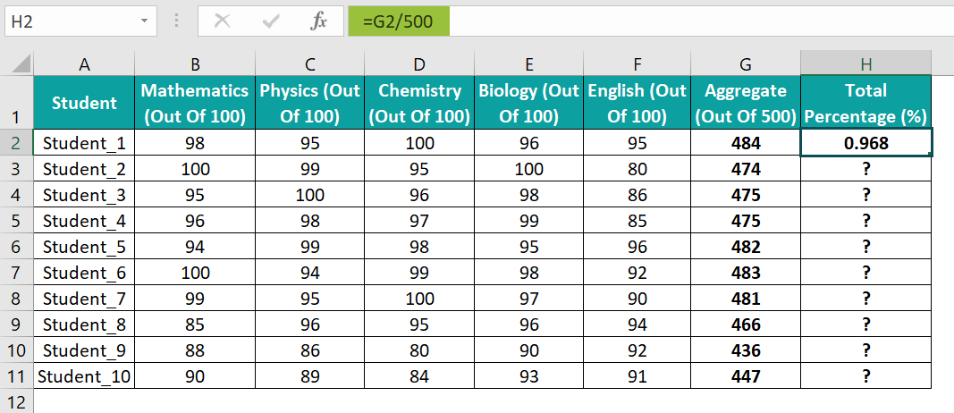
- Select the target cell H2, enter the formula =G2/500, and press Enter.
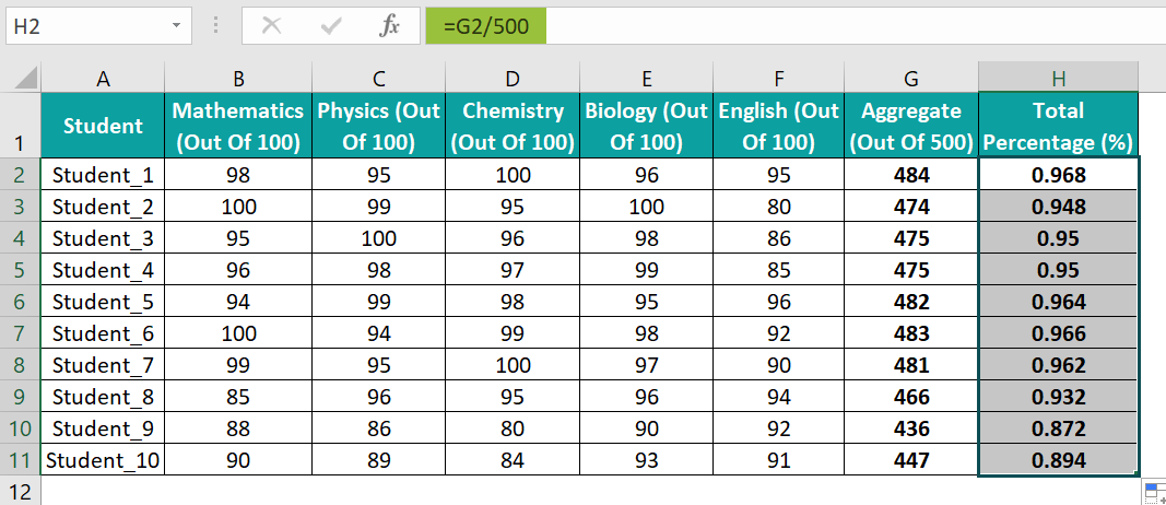
- Using the fill handle, drag the formula from H2 to H11.
- Select the cell range, H2:H11, and go to Home → Number Format → Percentage to view the values as percentages.

And once we click the Percentage format, the output is as shown below.
[Alternatively, select the target cells H2:H11, right-click to open the context menu, and pick the Format Cells option.
In the Format Cells window, click the Percentage category in the Number tab, and set the required decimal places as 2 to get the output in the desired percentage format. Then, click “OK” to close the dialog box.
Thus, as per the chosen Percentage format, cell values are in percentage values up to two decimal places.

Examples
We will see scenarios for the Percentage in Excel and use the option in the best possible ways.
Example #1
The below example shows how to increase by Percentage in Excel, and the formula to use in such a case is: =number * (1 + percent_increase)
Here, the number is the value to which we must add Percentage in Excel.
The following table contains a set of stocks and their prices. We will update the percentage increase in each stock price in column D. And determine the revised stock prices in column E after adding the percentage increase in the price of each stock to its corresponding initial price.

The steps to perform the required calculations and get the results in percentage format are,
- Step 1: Select cell range D3:D7, and press the keys Ctrl + Shift + % or Home → Number Format → Percentage to set the cell format as Percentage.

- Step 2: Enter the required values in cells D3:D7 that we want to view as percentages.

Alternatively, entering the required value followed by the ‘%’ symbol will automatically update the cell format as Percentage. We will not require to pre-format the cell as explained above.
- Step 3: Select the target cell E3, enter the formula =C3*(1+D3), and press Enter.

- Step 4: Use the fill handle to implement the formula in cells E4:E7.

- Step 5: Select the target cell range E3:E7, and set the Number Format in the Home tab as Currency to view the revised prices as currency values.

The output is shown below.

[Output Observation: Let us consider the cell E7 expression to check how the formula works.
=C7*(1+D7)
=2000*(1+0.19)
=2000*(1.19)
=2380
The above calculations imply that though Excel displays a percentage value, it considers the value’s decimal equivalent when performing calculations.
And once we update the cell E7 format as Currency, the revised price of the given stock is $2,380.]
Example #2
In the previous example, we saw how to add Percentage in Excel. Now, we shall see how to subtract a Percentage in Excel.
The table below shows a list of the top laptops and their prices.

Suppose the requirement is to update the discount rates and sales tax percentage of 8.25% in columns C and D. And to calculate each laptop price after the discount in column E. But we require to consider the sales tax while evaluating the result.
The steps to use the Percentage format in columns C and D and apply the required formula in column E to achieve the required data are,
- Step 1: Select the cell range C2:C6, and click the Percent Style icon in the Home tab to set the cell format as Percentage.

- Step 2: Update the required numbers in cell C2:C6, i.e., cells we want to view as discount percentages.

- Step 3: The sales tax value is 8.25%. And applying the default Percentage format will display the value up to 0 decimals, 8%. So, we must change the decimal places settings. And for that, we can select the cell range D2:D6, and press Ctrl + 1 to open the Format Cells window.

And pick the Percentage Category in the Number tab, as depicted above.
- Step 4: Set the Decimal places as 2, and click OK to close the window.

- Step 5: Enter the value 8.25 in cells D2:D6 to display the sales tax values.

- Step 6: Select the target cell E2, enter the formula =(B2*(1+D2))*(1-C2), and press Enter.

- Step 7: Using the excel fill handle, drag the formula to cells E3:E6.

- Step 8: Select the cell range E2:E6, and set the Number Format in the Home tab as Currency to get the final price values in currency.


The above formula first adds the sales tax percentage to the initial price, and then deducts the discount rate from the resulting amount to return the final price.
Further, to verify the discount % on each laptop, we can apply the discount formula within the ABS excel function and set the target cells’ format as Percentage.
Let us first introduce a new column in the above table to show the discount % for verification.

- Step 9: Select cell F2, enter the formula=ABS(E2/(B2*(1+D2))-1), and press Enter.

- Step 10: Use the fill handle to drag the formula to cells F3:F6.

- Step 11: Select the cell range F2:F6, and press the keys Ctrl + Shift + % to set the data format as Percentage.

Thus, we can compare columns C and F values to verify the discount percentage on each laptop model.
Example #3
The below table shows a set of items and their initial and final prices. We will update the percentage change in their prices in column D. Then, as some percentage values will be negative, we can show them using a customized percentage format.

The steps to perform the required calculations and get the results in percentage format are,
- Step 1: Select the cell range D2:D6, and follow the path Home → Number Format → More Number Formats…., as shown below, to open the Format Cells window.

- Step 2: In the Format Cells window, pick the Custom category in the Number tab, and enter the required percentage format under Type, as depicted below. And click OK to confirm the custom setting.
[Note: The specified custom percentage format shows negative percentages in red and up to two decimal places. On the other hand, the format will not apply to positive percentages, and they will display as it is.]

- Step 3: Select the target cell D2, enter the formula =(C2-B2)/B2, and press Enter.

- Step 4: Using the fill handle, drag the formula to cells D3:D6.

While all the target cells show the percentages in red, cell B4 is an exception. The reason is that the specified custom percentage format only applies to negative percentages and not to positive values.
Important Things To Note
- When applying the format for Percentage in Excel in a cell, ensure the cell contains a valid number or a formula returning a valid number.
- We can use the functions like IF in excel and IFERROR in excel to overcome percentage errors.
- We can pre-format a cell with the Percentage format or enter the value in a cell and then apply the Percentage format in the cell to view the entered value as a percentage.
Frequently Asked Questions (FAQs)
There is no Percentage function in Excel. However, we can apply the Percentage number format in a required cell to show its value as a percentage.
The Percentage format in Excel behaves in the following way when applied in an empty cell. Let us understand the scenario with an example.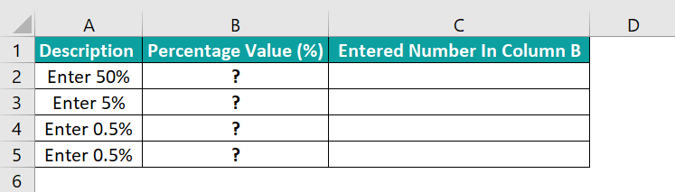
The steps to apply the Percentage format on empty cells are as follows:
• Step 1: Select cell range B2:B5, and navigate the path Home → Number Format → More Number Formats to open the Format Cells window.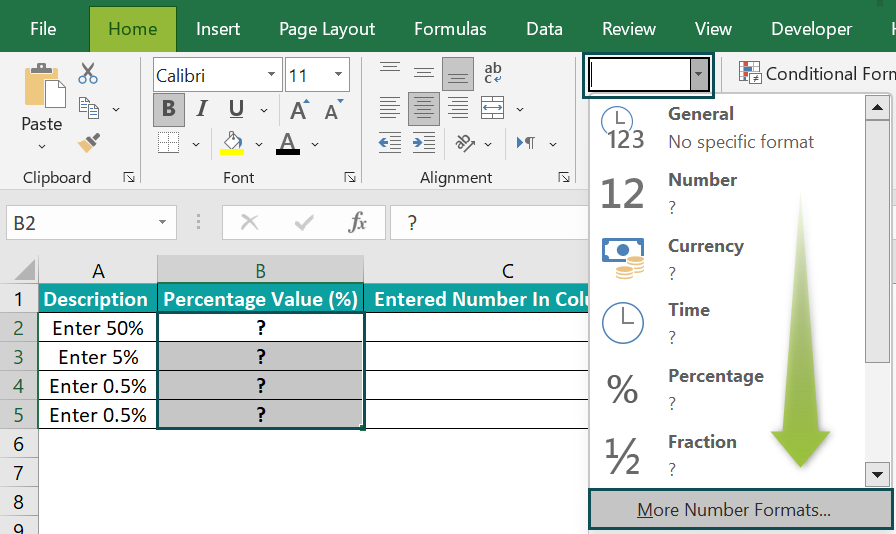
• Step 2: In the Format Cells window, set the Category as Percentage in the Number tab. Fix the decimal places as 1 to show percentages up to one decimal place. Click OK to apply the selected format.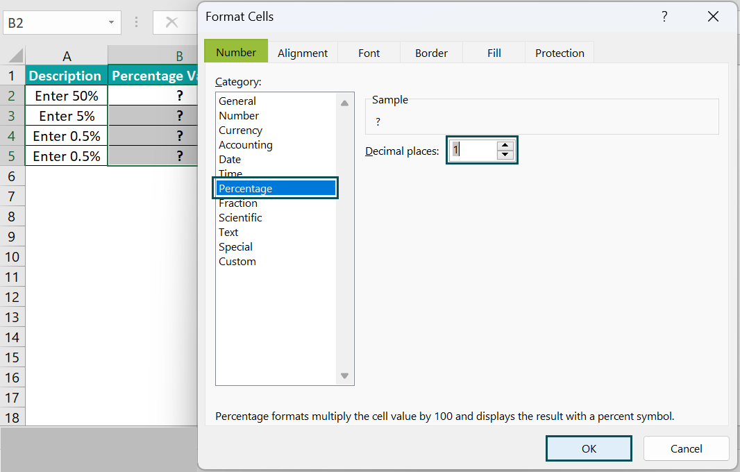
• Step 3: Select the target cell B2, and enter the first value as 50.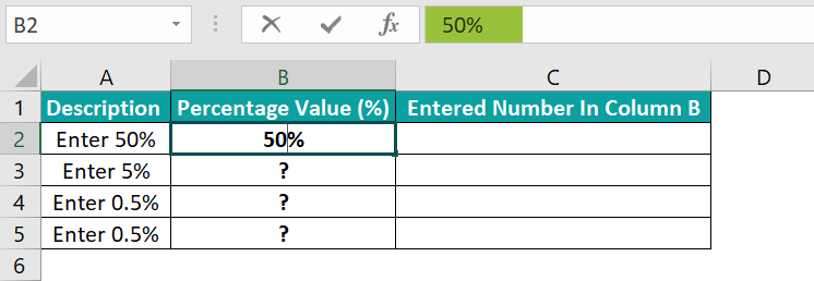
And press Enter to view the percentage value.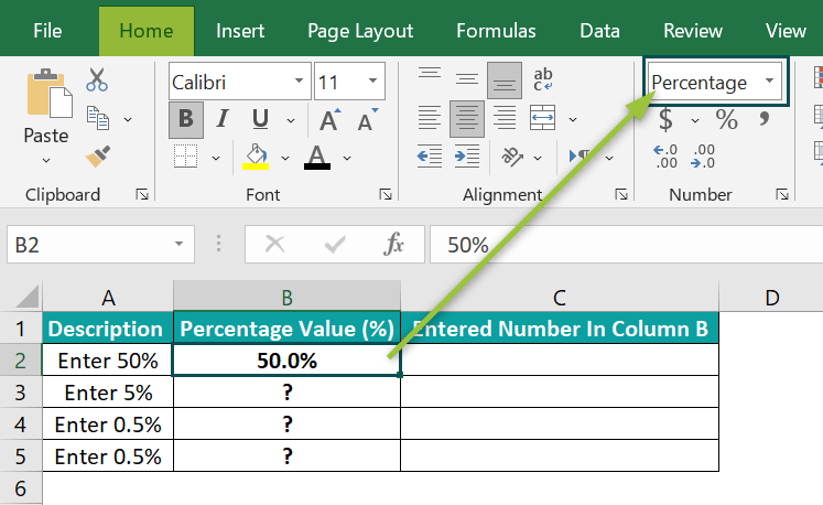
• Step 4: Enter the required values in the remaining target cells B3:B5.
Column C shows the values we entered in the target cells.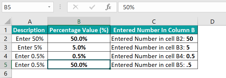
As per the requirement, the target cells B4:B5 should show the same value, 0.5%. But, while cell B4 shows the required percentage, cell B5 displays an incorrect value. The reason is that applying the Percentage format before entering a value in a cell treats the value differently.
If the supplied value equals or exceeds 1, the pre-format setting displays it as a percent. And if the value is less than one and entered without a preceding zero, the number gets multiplied by 100, as in the row 5 target cell. The value .5 gets multiplied by 100, and we see a value of 50% instead of the correct value of 0.5%.
On the other hand, the value entered in cell B4 is a number less than one but with a preceding zero. So, we see the correct percentage in cell B4.
Few reasons that the Percentage in Excel may be incorrect are,
• The data format of the supplied value is Text.
• The formula return value in the cell where we applied the Percentage format is invalid or inaccurate.
• We did not apply the appropriate Percentage format.
• The cell format is already Percentage, but we multiply the cell value by 100.
Use this Percentage In Excel Template to follow along with the examples in this article.
Download Excel Template