What Is Change Data Source For Pivot Table?
The Pivot Table Change Data Source is an option to update the data additions and deletions made to the source dataset in the Pivot Table. We can access the option from the Analyze tab in the ribbon.
Users can use the Pivot Table Change Data Source option when working with dynamic finance data, based on which we must update the inserted Pivot Table.
📥Download the ready-to-use Excel template to practice this tutorial yourself.
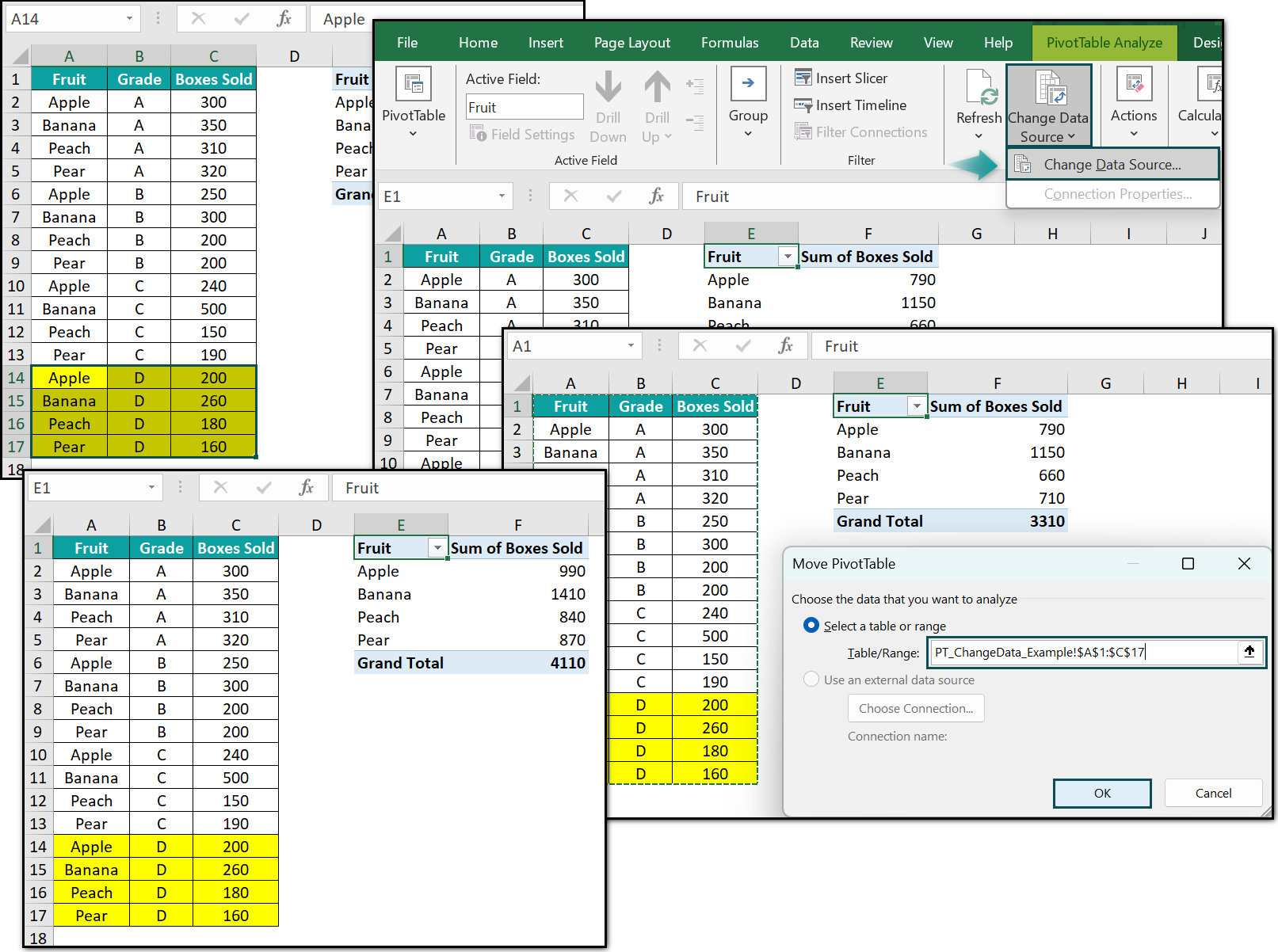
Pivot Table Change Data SourceFor example, the following image shows a source dataset in the range A1:C13 and an Excel Pivot Table in the range E1:F6 based on the source dataset.

While the source dataset lists fruits, their grades and boxes sold data, the Pivot Table lists the fruits and the total number of boxes sold data for each fruit based on the source data.
Let us consider that we add a new set of Grade D fruits’ data to the source dataset in the range A14:C17, and we must update the new data in the Pivot Table.
Then, we can perform this using the Change Data Source option in the Analyze tab.

In the above example, we click on a cell in the Pivot Table to enable the Analyze tab in the ribbon. Next, choose the Change Data Source option under the Change Data Source command in the Analyze tab.
The Change PivotTable Data Source window opens, showing the initial source dataset range in the Table/Range field. We shall click in the Table/Range field and then choose the cell range A1:C17 to update it as the new source dataset range to include the newly added data in the Pivot Table.
The above step will change the Change PivotTable Data Source window name to Move PivotTable.
Finally, clicking OK in the Move PivotTable window will update Pivot Table change data source, with the cells F2:F6 data in the Pivot Table confirming the same.
Thus, since we changed the Pivot Table’s data source, the Pivot Table shows the updated total number of boxes of each fruit sold based on the new source dataset.
Table of contents
Key Takeaways
- The option for Pivot Table change data source enables us to update the Pivot Table based on the rows and columns of data added to or removed from the source dataset.
- Users can use the option to change the Pivot Table’s data source when working with Pivot Tables based on financial data involving frequent changes in data ranges.
- We can use the Change Data Source option in the Analyze tab to manually change a Pivot Table’s data source. Otherwise, we can use VBA coding to perform the same action.
How To Locate The Data Source Of Pivot Table?
The steps to locate a Pivot Table’s data source are as follows:
- Click a cell in the Pivot Table, created based on the given source dataset, to enable the Analyze tab in the ribbon.

- Choose the Change Data Source command down arrow → Click the Change Data Source option in the Analyze tab.

- The Change PivotTable Data Source window will open, showing the source data range in the Table/Range tab based on which we created the Pivot Table.

[ Alternatively, we can click in the Pivot Table and use the change data source shortcut, Alt + JT + I + D. The shortcut will help us access the Change PivotTable Data Source window and view the corresponding Pivot Table’s data source.]
How To Change Data Source In Excel Pivot Table?
While we can use the VBA Pivot Table change data source to change a Pivot Table’s data source, we shall see the more straightforward methods to perform the required action.
#1 – Change Data Source Of Pivot Table
The steps to change a Pivot Table’s data source using the update Pivot Table Change Data Source option are as follows:
- Ensure the new data added to the existing source dataset or the rows of data removed are aligned with the requirements.
- Click on a cell in the Pivot Table, created based on the initial Pivot Table, to enable the Analyze tab in the ribbon.
- Choose the Change Data Source command down arrow → click the Change Data Source option in the Analyze tab.
- The Change PivotTable Data Source window will open, showing the initial source dataset range in the Table/Range field, based on which we created the Pivot Table.
- Update the new source dataset range in the Table/Range field.
- The window name changes to Move PivotTable. Click OK in the Move PivotTable window to view the updated Pivot Table.
Thus, the refreshed Pivot Table includes the data we added to the initial source dataset or excludes the data we deleted from the source dataset.
Basic Example
The following image shows a source dataset in the range A1:C10 and a Pivot Table in the range E1:F5 based on the source dataset.

The source dataset lists employees and their time to complete the tasks.
Let us consider that we must change the cells C7:C8 data and append new data for another task in the range A11:C13 in the source dataset, as highlighted below.

Then, the Pivot Table does not refresh automatically to reflect the source dataset changes. So, here is how to manually update the changes in the Pivot Table.
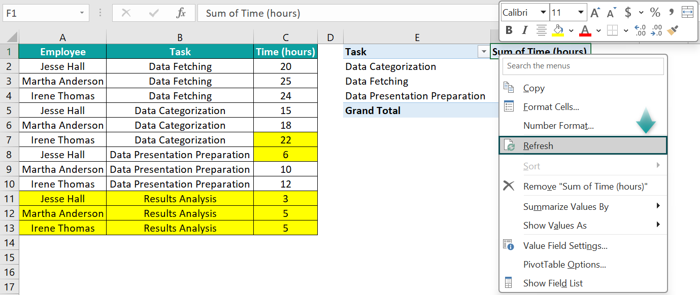
- Step 1: Right-click a cell in the Pivot Table to open the context menu and choose Refresh from the menu.


The Pivot Table updates the values we changed in cell C7:C8. However, it does not reflect the newly added data to the source dataset.
Thus, instead of using the Refresh option, we can directly use the Change Data Source option to update the value changes and new data additions in the Pivot Table in one go.
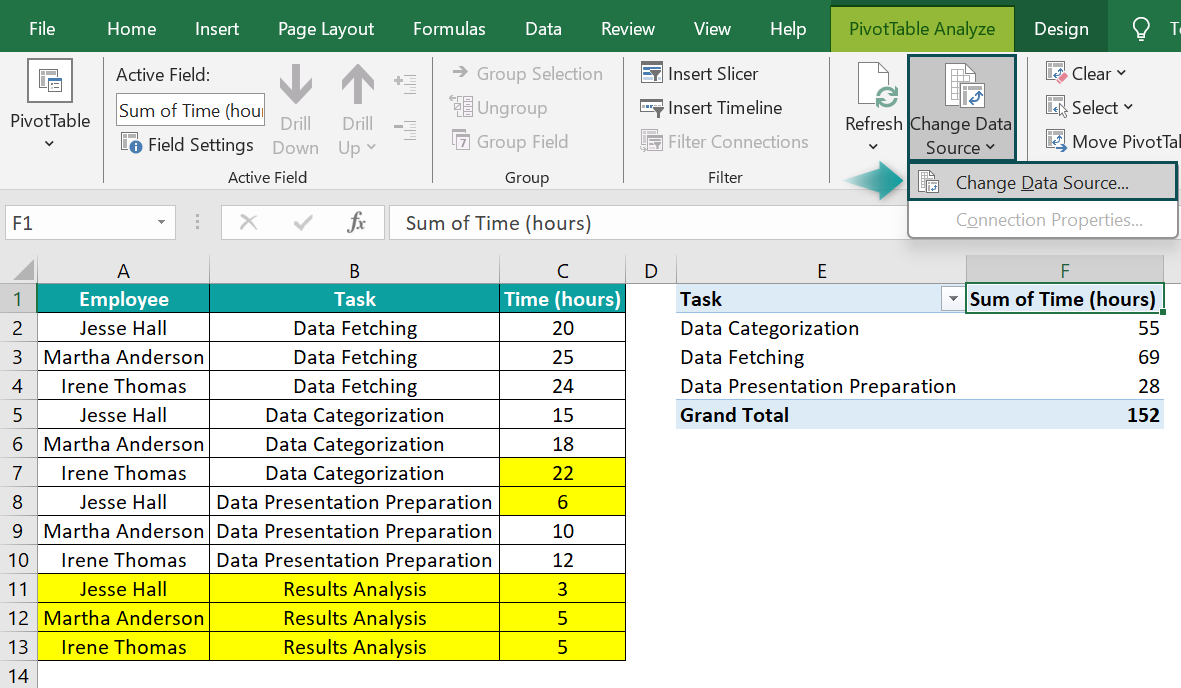
- Step 2: Click a cell in the Pivot Table to enable the Analyze tab and choose the Change Data Source command down arrow → Change Data Source option.

[ Alternatively, click a cell and use Alt + JT + I + D as the Excel Pivot Table change data source shortcut.]
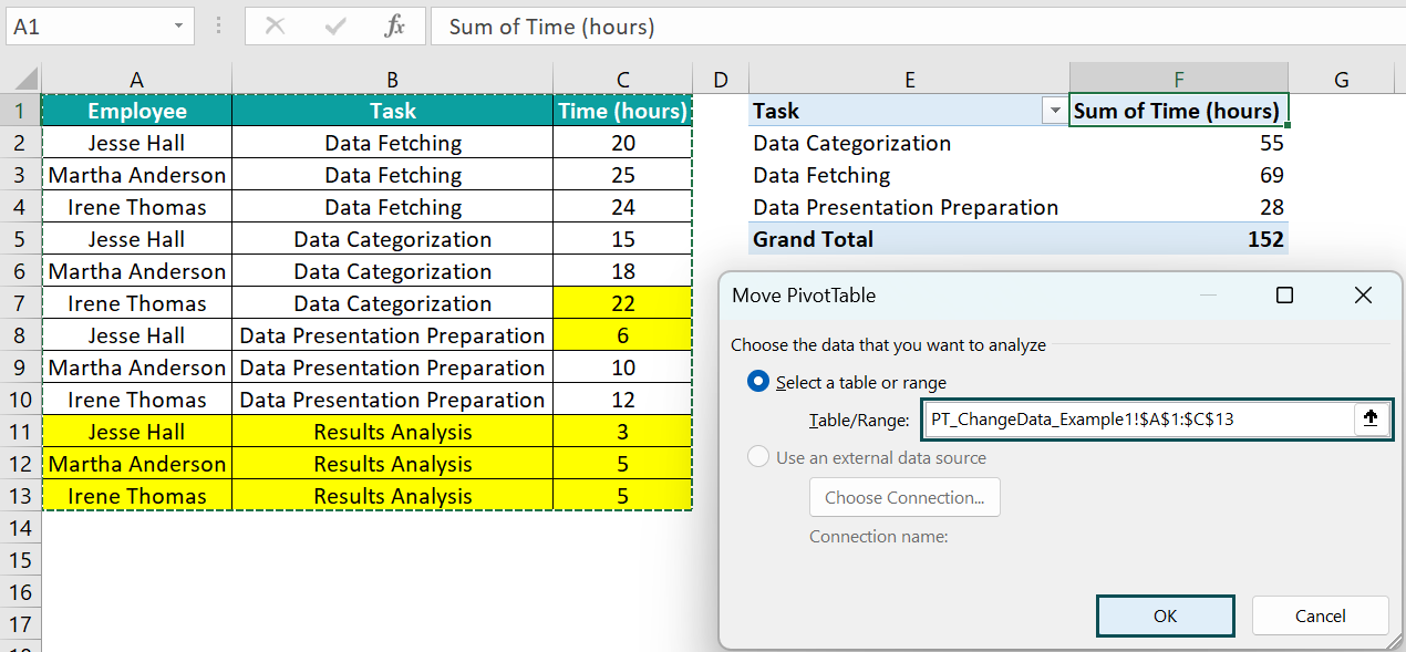
The Change PivotTable Data Source window opens. It shows the source dataset range in the Table/Range field, based on which we created the Pivot Table.

- Step 3: Click the Table/Range field in the Change PivotTable Data Source window and select the new source dataset range in the sheet.

While the window name changes to Move PivotTable, the Table/Range field shows the source dataset range, including the newly added data.
Finally, clicking OK in the Move PivotTable window will update the Pivot Table.

Thus, the updated Pivot Table shows the task details we added recently in the source dataset.
While we can use the VBA Pivot Table change data source option to achieve the required result, the above method is a quicker and easier alternative.
#2 – Auto Data Range Source Of Pivot Table
Sometimes, we may create a Pivot Table based on an Excel Table.
In such a scenario, the auto data range source of the Pivot Table is possible. We can change the data source for a Pivot Table using the Refresh option for data additions and deletions in the source Excel Table.
So, here is how to perform the required auto data range source of Pivot Table:
- Ensure the new data we add to or delete from the source Excel Table is aligned with the requirements.
However, if the new data does not appear in the same format as the Excel Table, select the File tab and choose Options.


The Excel Options window opens. Click the Proofing tab to open it and choose AutoCorrect Options in the Excel Options window.

The AutoCorrect window opens, where we must click the AutoFormat As You Type tab to open it. Next, select the option to include new rows and columns in the table under the Apply as you work heading.

Click OK to exit from the window.

Finally, click OK in the Excel Options window to apply the changes in Excel.
Hence, now we can add new rows and columns of data to the existing Excel Table.
- Right-click a cell in the Pivot Table, created based on the initial source Excel Table, and select the Refresh option from the contextual menu.
We will see the updated Pivot Table, showing the data we added to the initial source Excel Table.
Basic Example
The following image shows a source Excel Table in the range A1:C13 and a Pivot Table in the range E1:I7 based on the Excel Table.

The source Excel Table lists students and their project points in different subjects.
Let us consider that we update the project points of a student, Gary Nelson, in English from 42 to 48 in cell C9. Also, we append another subject data to the existing Excel Table in the range A14:C17.

Then, here is how to update the value change and the change in the data source in the Pivot Table.
- Step 1: Right-click a cell in the Pivot Table and select Refresh from the contextual menu.

While the Pivot Table will show the updated English project points of Gary Nelson, it will also include the new subject data, as shown in the image below.

Important Things To Note
- The keyboard shortcut to access the Change PivotTable Data Source window to perform the Pivot Table change data source is Alt + JT + I + D.
- Ensure the data source range reference we enter in the Table/Range field in the Change PivotTable Data Source window is valid and correct. Otherwise, the data source range of the Pivot Table will update incorrectly and may result in an error.
- If the source dataset is an Excel Table, we can use the Refresh option to change the data source of the Pivot Table created based on the Excel Table.

Frequently Asked Questions (FAQs)
We can change Pivot Table data source using VBA in the following way, explained with an example.
The image below shows a source dataset containing a list of products, their categories and sales figures in one worksheet.
Further, we have a Pivot Table based on the source dataset in another worksheet, with the PivotTable Name field in the Analyze tab showing the Pivot Table name as PivotTable5.
Here is how to change the Pivot Table data source using VBA.
• Step 1: Open the worksheet containing the source dataset and press Alt + F11 to access the VBA Editor.
• Step 2: Expand the applicable VBAProject, right-click the worksheet containing the source dataset and choose the View Code option from the popup menu.
The corresponding coding window opens.
• Step 3: Enter the VBA code to change the Pivot Table data source.
• Step 4: Open the source dataset worksheet and add the required new product data. In this example, we add the new data in the range A12:C13, highlighted in the image below.
• Step 5: Go to the worksheet containing the Pivot Table, where we will find the data source changed for the Pivot Table, and it includes the data added newly to the source dataset.
You can’t change data source on Pivot Table, perhaps because of the following reasons:
• The Pivot Table is based on a Workbook Data Model.
• The data source range reference you are trying to update in the Table/Range field in the Change PivotTable Data Source window is incorrect or invalid.
We can change Pivot Table data source Google Sheets using the following method:
1) The Pivot table editor shows the data source. But If the editor is not visible, click the Edit button below the pivot table.
2) Click the Select data range icon (⊞) to show the Select a data range dialog box.
3) Click on the worksheet containing the updated source data and select the entire range.
4) Finally, click OK to update the pivot table according to the data source changes.
Download Template
📥Download the ready-to-use Excel template to practice this tutorial yourself.
Pivot Table Change Data SourceRecommended Articles
This has been a guide to What Is Pivot Table Change Data Source. We learn to locate and change the data source of pivot tables in Excel with examples. You can learn more from the following articles –


Leave a Reply