Sparklines in Google Sheets

What Are Sparklines in Google Sheets?

The Sparkline function in Google Sheet allows you to build small charts in a cell to depict the trend of the selected data range. This miniature chart is small and does not usually contain axes. It is present inside a cell. Sparklines can take the form of a line, bar, or column chart. Sparklines can be used with numerical data in a tabular format. 

Look at the below example of how a trend line has been plotted for the given values. The SPARKLINE function in Google Sheets formula to create a miniature chart is as shown in the image. 

In this article, let us look into all the details regarding the plotting of a Sparkline in Google Sheets.

How to Insert Sparklines in Google Sheets

Let us look at how to create these miniature charts in Google sheets. For any regular chart in Google Sheets, you go to Insert => Chart. However, to create sparklines, you specify the required parameters in the formula. Before we look at how to insert sparklines, let us look at the syntax and different available options.

SPARKLINE Syntax

=SPARKLINE(data-range, {option1,option1-value;option2,option2-value,…})

• data-range – it specifies the data range for which you want to create the SPARKLINE.
• option – includes the options for the sparkline chart.
• option-value – the value associated with the option
  • The “charttype” option defines the type of chart to plot, which includes “line” for a line graph, “bar,” “column” for a column chart, and “winloss” for a special type of column chart.
  • ‍For line graphs, you have special options like “xmin,” “xmax,” “ymin,” “ymax,” “color,” etc.
  • For bar charts, there is “max,” “color1,” “color2,” etc.

Let us look at the steps to insert a sparkline chart. Some data in a Google sheet is given below. We have also listed the number of items purchased by customers at a stationary shop.

Here, we have empty cells as well. Let us look at how to deal with it. We’ll choose two options to build the sparklines. 

Step 1: Enter the following formula in cell B8.

=sparkline(B2:B7,{ “charttype”,”column”;”empty”,”zero”})

Step 2: Press Enter. You can see a column graph with the empty cell typically represented as a zero.

You can see that the parameters can completely change how your sparkline looks.

Types of Sparklines in Google Sheets

Let us look at the types of sparklines in Googles Sheets. We can also look at some simple examples for each type to understand in detail how sparklines work.

• Line graph
• Column chart
• Bar chart
• Win/loss column chart

#1 – Line Sparklines

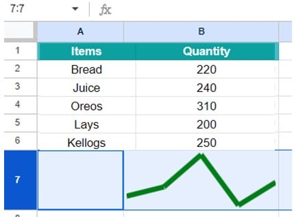
Line sparkline is the default type of miniature chart, which is displayed by Google Sheets when we create a sparkline. So, we do not use the “charttype” option. You can customize this graph the way you want. The number of items stocked at a supermarket is given below.

Step 1: Let us plot the line graph. Use the following formula in cell B7.

=SPARKLINE(B2:B6, {“color”,”green”})

Step 3: You can draw the line graph with different options and get amazing results. Enter the formula in cell B7. Here, we change the line width.

=SPARKLINE(B2:B6, { “color”,”green”;”linewidth”,6})

#2 – Column Sparkline

To create a column chart, you must specify the option as {“charttype”, “column”}. Let us look at how to create a column chart. Let us look at some data which describes the loss or profit after a sale. A negative sign gives the loss.

Step 1: Let us apply the following formula for the column sparkline. Apply it in cell B7.

=SPARKLINE(B2:B6,{“charttype”,”column”;”color”,”blue”})

Step 2: Here, we specify the chart type as column and the color as blue. Press Enter.

Step 3: As seen above, the negative values appear below the axis. Let us set the axis to be visible with a color.

=SPARKLINE(B2:B6,{“charttype”,”column”;”color”,”blue”;”axis”, true;”axiscolor”,”maroon”})

Here we give the axis to be visible(true) and its color as red.

Apply the above formula in cell B8.

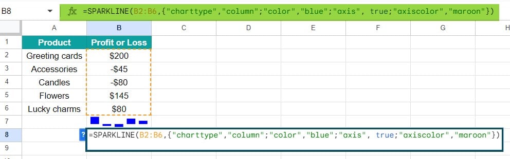
Step 4: Press Enter. You can see the axis in red. Thus, the sparkline in Google Sheets is a pretty helpful tool that helps you analyze the data at a glance. 

#3 – Win-Loss Sparkline 

Next, let us look at the Win-Loss sparkline. If you’re curious to know what it is, you should understand that it is a simplified version of the column chart. In a column chart, the height varies based on the values in the supplied data range, whereas in a win-loss sparkline, columns are equally sized and only differentiate between positive and negative values. To give the chart type as Win-Loss, you must give the following option in the formula. {“charttype”, “winloss”}

Let us look at a clear example to understand the difference. Look at the data below.

Step 1: Let us try to plot a Win-Loss sparkline. Use the following formula in cell C2.

=SPARKLINE(A2:A8,{“charttype”,”winloss”;””axis”, true;”axiscolor”,”black”})

Step 2: Press Enter. You will observe that the negative values are below the axis while the positive are above. 

Step 3: You can use different colors for the bars of positive and negative values, as follows. Change the formula as follows.

=SPARKLINE(A2:A8,{“charttype”,”winloss”;”axis”,true;”axiscolor”,”black”;”negcolor”,”red”})

Step 4: We will use the column chart to show the difference between Win-Loss and the column chart. Just change the chart type to column.

=SPARKLINE(A2:A8,{“charttype”,”column”;”axis”,true;”axiscolor”,”black”;”negcolor”,”red”})

#4 – Bar Sparklines

The bar sparklines are usually used when they have a maximum of two values in a column/row. It uses only two different colors to differentiate between the values. Given below is a sale of computers at a store over two months.

Step 1: Let us apply the formula for the third row. Remember, we have to apply seven separate SPARKLINE formulas for each row.

=SPARKLINE(A3:B3,{”charttype”,”bar”})

Apply the above formula to cell C3.

Step 2: Press Enter. Apply the formula repeatedly from C3 to C9. Only changing the ranges as A4:B4, A5:B5, etc. You will get charts as shown below. 

How to Change Sparklines in Google Sheets?

Changing a sparkline in Google sheets is simple. Let us look at one of the previous examples of a column sparkline.

Let us try to change this to a win-loss chart and apply colors. To do so all you have to do is to change the chart type and customize all the necessary options. Here, I would like to change the color of the bars and also convert it to a win-loss chart. The previously used column chart sparkline formula in Google sheets was:

=SPARKLINE(B2:B6,{“charttype”,”column”;”color”,”blue”})

Now, we will change to a win-loss chart and differentiate the sparkline bar google sheets. Apply the formula below with changes.

=SPARKLINE(B2:B6,{“charttype”,”winloss”;”highcolor”,”blue”;”lowcolor”,”pink”,”lastcolor”,”green”;”negcolor”,”yellow”}).

#1 – Resize Sparklines

The generated sparklines are usually very tiny for you to make complete sense of them. However, you can resize them in two ways. Let us look at one of our previous graphs.

1. Drag the width of the cell with your mouse.

• Select the particular column and row. Right-click and choose the Resize row/Resize column option and enter appropriate values.

#2 – Delete Sparklines

Deleting sparklines does not have any function in Google sheets. You just delete the formula by clicking on the particular cell and the sparkline is deleted.

Important Things To Note

• Sparklines in Google sheets consider numeric data and ignore non-numeric data.
• A line sparkline can only have one color, while a bar sparkline can only have two colors.
• If you change the cell dimension of a sparkline, the chart adjusts itself accordingly to fit within the cell.
• You can nest a QUERY formula into a SPARKLINE formula to merge many sparklines into one. For this, you must combine the data ranges into one.
• Numerous options are available in Google Sheets for various sparkline chart types to produce a colorful, easy-to-understand chart.

Frequently Asked Questions (FAQs)

Recommended Articles

Guide to Sparklines in Google Sheets. Here we explain How to insert Sparklines in Google Sheets with its types and how to change it. You can learn more from the following articles. –

• Venn Diagram in Google Sheets
• Data Validation In Google Sheets
• Exponential Function in Google Sheets