What Is Excel SUMIF Text Function?
The Excel SUMIF Text function is a powerful tool that allows users to calculate the sum of values in a range based on specified criteria. Unlike the regular SUMIF function, which only accepts numerical values, the SUMIF Text function works with text or alphanumeric characters. It evaluates the cells in a given range and adds up only those cells that match the specified criteria. This function is particularly useful when dealing with data that contains both text and numbers, as it enables users to perform calculations based on specific text conditions.
In this example, we will explore the amazing SUMIF Text Excel function, which is a nifty tool for calculating specific values based on certain criteria. Our ultimate goal is to figure out the total in Thousands of “G” words in a given scenario.
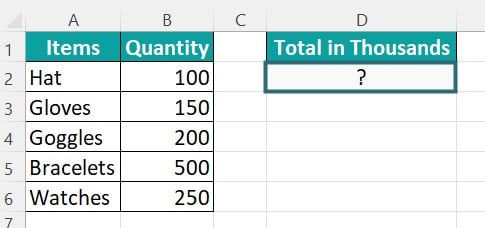
To get started, simply choose the cell where you want the formula to work its magic and show the final result. For this demonstration, let’s go with cell D2. Take your time and enter the formula exactly as shown below: =SUMIF(A2:A6, “*G*”, B2:B6).
The resulting value will automatically pop up in cell D2. If you need a visual representation of what to expect, just refer to the provided image.
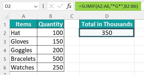
Table of Contents
Key Takeaways
- The SUMIF function is a conditional function in Excel that allows for the summation of cells based on specific criteria, including text. This powerful tool enables users to easily sum up a group of cells that meet a particular text-based condition.
- The SUMIF function is one of the many built-in mathematical and trigonometric functions available in Excel. With its ability to perform conditional summation, it proves to be an invaluable asset for data analysis and calculation purposes.
- In the realm of Excel, the SUMIF function becomes particularly useful when we need to sum numbers within a range of cells, depending on specific text criteria. What sets this function apart is its indifference towards the case of the text, making it even more versatile and user-friendly.
Syntax

- Range – This parameter is mandatory as it defines the values or range of cells that need to be tested against the specified criteria.
- Criteria – Another mandatory parameter represents the condition that will be checked against each value within the supplied range.
- Sum_range – This parameter is optional. It allows you to specify the values or range of cells that should be added together if the “range” parameter meets the given condition or criteria. If this parameter is not provided, Excel will automatically sum the cells specified in the range argument itself.
How To Use Excel SUMIF Text Function? (With Steps)
To effectively utilize the SUMIF function in Excel, follow these steps.
#1 – Access From The Excel Ribbon
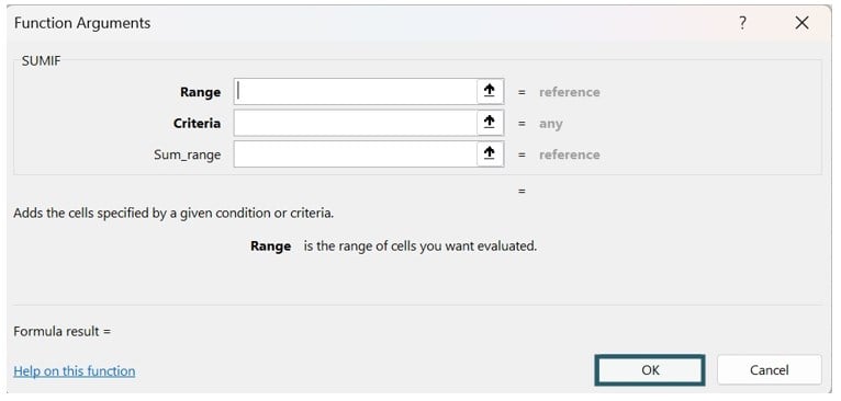
Step 1: Choose the empty cell which will contain the result. Go to the Formulas tab and click it.

Step 2: Select the Math & Trig option from the menu.

Step 3: Select SUMIF from the drop-down menu.

Step 4: A window called Function Arguments appears. As the number of arguments, enter the value in the range, criteria, and sum_range.
Select OK.
#2 – Enter The Worksheet Manually
Step 1: Select an empty cell for the output. Type =SUMIF() in the selected cell. Alternatively, type =S and double-click the SUMIF function from the list of suggestions shown by Excel.
Step 2: Press the Enter key to get the result.
Examples Of SUMIF Text In Excel
Example #1
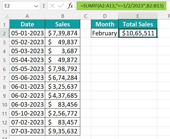
In the following example, we will explore and apply the concept of the SUMIF Text Excel function. Let’s calculate the total sales of February in the given scenario.
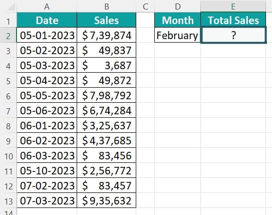
The data within the provided table is organized as follows:
To calculate the desired output in cell E2, please follow these steps:
Step 1: Choose the cell where you want to enter the formula and calculate the result. For this example, let’s use cell E2. Enter the formula exactly as shown below:
= SUMIF(A2:A13,“<=1/2/2023”,B2:B13).
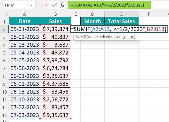
Step 2: After entering each value in the previous step, press the Enter key. As a result, you will see the corresponding value displayed in cell E2, just like in the provided image.
Example #2
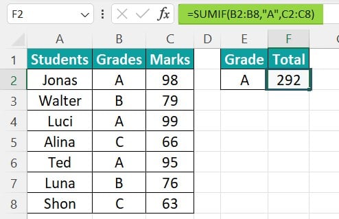
Let’s use the example and explore the SUMIF Text Excel function. We’ll be calculating the total marks of grade A students in a given scenario.
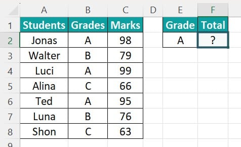
To facilitate matters, we have at our disposal a meticulously arranged table containing comprehensive data.
Step 1: First, choose the cell where you want to enter the formula and calculate the result. In this case, we’ll use cell F2. Now, enter the formula exactly as shown below:
=SUMIF(B2:B8, “A”, C2:C8).
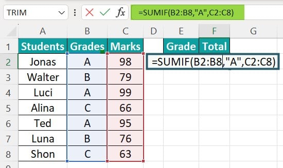
Step 2: Once you’ve entered the formula, press the Enter key. The corresponding value will be displayed in cell F2, just like in the provided image.
Example #3
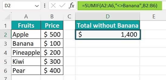
Let’s dive into an example and explore the SUMIF Text Excel function. We’ll be calculating the price of fruits without Banana in a given scenario.

To make things easier, we have a table with organized data.
Step 1: First, select the cell where you desire to input the formula and compute the outcome. In this instance, we will utilize cell D2. Now, meticulously enter the formula precisely as depicted below:
=SUMIF(A2:A6, “<>Banana”, B2:B6).

Step 2: The resulting value will be displayed in cell D2, similar to the example shown in the provided image.
Important Things To Note
- The SUMIF function is a built-in function in Excel that falls under the category of Mathematical/Trigonometric functions.
- The SUMIF function in Excel proves to be valuable when we need to sum numbers within a range of cells based on specific text criteria.
- However, it is important to note that if the “criteria” parameter provided to the SUMIF function exceeds 255 characters in length, the function will return the #VALUE! Error.
- In cases where we need to calculate the sum of values within a range based on multiple criteria, the SUMIFS function is the appropriate choice.

Frequently Asked Questions (FAQs)
The SUMIF Text function in Excel serves the purpose of summing values based on a specified criterion but with additional flexibility.
For example, our goal is to determine the total scores of Post Graduates in a given scenario as shown in the below image.
First, select the cell F2 and enter the formula: =SUMIF(B2:B7, “Post Graduation”, C2:C7).
Once you’ve entered the formula, the resulting value will be automatically displayed in cell F2. You can refer to the provided image for a visual representation of the expected outcome.
The SUMIF Text function, commonly used in Excel, does not differentiate between uppercase and lowercase text. This function allows users to sum values in a range based on a specified criterion. However, when using the “text” criterion, it treats all text entries as case-insensitive. This means that regardless of whether the text is uppercase or lowercase, the SUMIF Text function will consider them as equal and include them in the summation calculation.
The SUMIF function, typically used in spreadsheet software like Microsoft Excel or Google Sheets, allows users to sum a range of cells based on specified criteria. While SUMIF is a powerful tool for numerical criteria, it does have limitations when it comes to text criteria.
One limitation is that the function only supports partial matches with wildcards. For example, if “apple” is one of the text criteria, the function will not consider cells containing “apples” or “pineapple.”
Download Template
This article must help us understand the SUMIF Text Excel Function’s formula and examples. You can download the template here to use it instantly.
Recommended Articles
Guide to SUMIF Text In Excel. Here we learn how to use excel SUMIF text function with step by step examples using syntax and a downloadable template. You can learn more from the following articles –

Leave a Reply