Transpose In Google Sheets

What Is Transpose In Google Sheets?

Transpose in Google Sheets is a technique to switch data given in columns to rows and vice versa in Sheets. We can use the Paste special option, the inbuilt Array function TRANSPOSE, and other inbuilt functions with the TRANSPOSE() to transpose the given data in Google Sheets.

Users can utilize the methods to transpose in Google Sheets to change the orientation of the specified data in Sheets automatically.

For example, the source dataset contains a store’s annual inventory levels in columns A and B.

The requirement is to show the source dataset in rows 1 and 2. Assume, the target cell range starts from cell D1.

Then, considering the definition of transpose in Google Sheets explained earlier, we can use the Paste special option, which is similar to the Excel Paste Special option, to interchange columns of data into rows of data.

In this transpose data in Google Sheets example, we choose the cell range A1:B7 and copy the data by using the shortcut Ctrl + C. 

Next, select the first target cell D1. After that, right-click to choose the Paste special option right arrow in the pop-up menu and then the Transposed option.

The above action will transpose data in Google Sheets from the columns A and B cell range to the rows 1:2 cell range, with the source dataset format applied to the target cells.

How To Transpose In Google Sheets?

Aligning with the meaning of transpose in Google Sheets explained earlier, we can use the following three techniques to achieve the desired result.

1. Paste Special Option
2. TRANSPOSE Function
3. TRANSPOSE Function With Other Functions

#1 – Transpose In Google Sheets With Paste Special

We can use the Paste special option to perform Google Sheets transpose rows to columns and vice versa, as explained below:

1. Select the source dataset range. Next, right-click to choose the Copy option from the pop-up menu to copy the data. 
2. Select the target cell. Next, right-click to select the Paste special option right arrow – The Transposed option from the pop-up menu.

We shall see the transposed data in the target range, with the same format as the source dataset. 

However, the transposed data will be static. It implies that if we edit any data in the source dataset, we must delete the transposed data and repeat the entire copying and pasting process to view the modified data in the required orientation.

#Basic Example

The source dataset contains a person’s annual income and savings data in columns A to C cells A1:C8.

We need to change the source dataset’s vertical orientation to a horizontal orientation, with the target cell range starting from cell E1. Then, the steps are as follows:

Step 1: Choose the source dataset range A1:C8.

Next, right-click to choose the Copy option from the pop-up menu to copy the selected data.

Step 2: Choose the first target cell E1. Next, right-click to access the pop-up menu. After that, choose Paste special – Transposed from the pop-up menu.

Once we choose the Transposed option, we will see the transposed static data in the target range.

#2 – Transpose With Google Sheets TRANSPOSE Function

The steps to transpose with the Google Sheets TRANSPOSE function, which works like the TRANSPOSE in Excel, are as follows:

The TRANSPOSE function in Google Sheets syntax is the following:

Where,

• array_or_range: The mandatory argument, which is the array or cell range whose rows and columns of data will be switched.

We can utilize the function TRANSPOSE in Google Sheets in the following ways:

1. Access the function from the ribbon.
2. Enter the function into the sheet manually.

Method #1 – Access The Function From The Ribbon

Choose a target cell for showing the result – The Insert tab – The Function option right arrow – The Array function group right arrow – The TRANSPOSE function.

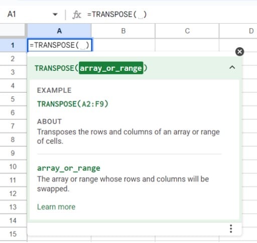
The chosen function will show in the target cell, with the cursor within the function brackets. We can now supply the function argument within the brackets.

Further, clicking the ‘?’ symbol on the left of the function name will show the function syntax.

We can then select the down arrow in the syntax pane to know the meaning of the TRANSPOSE function In Google Sheets described with a basic example.

Finally, press Enter to view the array of values or the transposed data the function TRANSPOSE in Google Sheets returns.

Method #2 – Enter The Function Into The Sheet Manually

1. Choose the target cell where we want to show the result.
2. Type =TRANSPOSE( in the cell. [ Alternatively, type =T or =TR and click the function name TRANSPOSE from the suggestions to select the function.]
3. Provide the argument value and close the brackets.
4. Press Enter to get the transposed data the function TRANSPOSE in Google Sheets returns.

In this case, the source dataset format will not be applied to the transposed data in the target cell range. 

However, the transposed data will be dynamic. So, if we edit the source dataset, the changes will be reflected in the transposed dataset.

#Basic Example

The source dataset shows a store’s monthly smartphone units sold data in columns A and B cells A1:B7.

We must swap the columns of data into rows of data, with the target range starting with cell D1. 

Then, we can apply the TRANSPOSE() in cell D1 to change the source dataset orientation.

Step 1: Choose cell D1 and enter the TRANSPOSE() preceded by the ‘=’ symbol.

The above action will show the function in the chosen cell.

Next, update the argument value in the function in line with the function syntax and close the bracket.

[Alternatively, select cell D1 and then Insert – Function – Array – TRANSPOSE.

The above step inserts the chosen function in the target cell.

Update the function argument value, as depicted above.]

Step 2: Press Enter to view the transposed array of values the TRANSPOSE() returns.

Step 3: Use the formatting options from the ribbon to view the transposed data in the desired format.

#3 – Use TRANSPOSE With Other Functions

We can apply the TRANSPOSE() as a standalone function. However, we can use the function with other inbuilt functions, such as UNIQUE and SPLIT, to achieve practical results.

The steps are as follows:

1. Select the range that we want to transpose.
2. Choose the target cell and enter the applicable formula containing the TRANSPOSE function with other functions.
3. Press Enter to view the formula output.

#Basic Example

The source dataset shows the zone-wise revenue data of the sales representatives at a firm. Also, cell B13 shows the zones separated by commas.

The aim is to display the unique zone values, cited in cells A2:A11, in row 1 cells, F1:I1. Also, we must display the zones cited in cell B13 individually in column K cells, K2:K5.

Step 1: Choose cell F1 and enter the TRANSPOSE() containing the UNIQUE().

=TRANSPOSE(UNIQUE(A2:A11))

Next, press Enter to view the unique zone values in cells F1:I1.

The UNIQUE() determines the distinct values in the input range A2:A11, which are North, South, East, and West. 

These values will be in a target cell and the cells below it, i.e., as a column of data. So, nesting the UNIQUE() within the TRANSPOSE() will swap the column of data into a row of data, which we see in cells F1:I1.

Step 2: Select cell K2 and enter the TRANSPOSE() containing the SPLIT().

=TRANSPOSE(SPLIT(B13,”,”))

The SPLIT() will show the values of the list, cited in cell B13, individually in the target cell and cells adjacent to it, i.e., as a row of data. So, nesting the SPLIT() within the TRANSPOSE() will swap the row of data into a column of data, which we see in cells K2:K5.

Thus, we see how to perform Google Sheets transpose rows to columns and vice versa using the TRANSPOSE() with other functions.

#4 – Use Shortcut To Transpose In Google Sheets

The steps to use a shortcut to perform the transpose operation in Google Sheets are the following:

1. Select the range of data we aim to transpose. Next, press Ctrl + C, which will copy the chosen data.
2. Select the first cell of the target range. Next, press Alt + E + S + E to paste special to the chosen data, with the copied data appearing transposed.

#Basic Example

The source dataset lists the date-wise prices of a stock in columns A and B cells, A1:B6.

The aim is to swap the source data from columns to rows with the target range starting from cell D1.

Step 1: Select cells A1:B6. Next, using the keys Ctrl + C, copy the data, following which we shall choose cell D1.

Step 2: Press Alt + E, which will show the Edit tab options. Next press S, which will show the Paste special options.

Finally, press E to choose the Transposed option from the Paste special options.

The above action will swap the chosen columns of data into the required rows of data, with the transposed data in the target cells in the same format as the source dataset.

Important Things To Note

• Ensure the argument value supplied to the TRANSPOSE() for performing transpose in Google Sheets is a range or array. Otherwise, the function output is the #N/A error.
• When we use the TRANSPOSE() as the Google Sheets transpose formula, the function syntax should be correct. Otherwise, the function output is the #NAME? error.
• When using the Paste special option as a transpose method in Google Sheets, the transposed data will be static and will have the same format as the source dataset. However, the TRANSPOSE() will result in dynamic transposed data without the source dataset format.

Frequently Asked Questions (FAQs)

Download Template

This article must be helpful to understand the Transpose In Google Sheets, with its formula and examples. You can download the template here to use it instantly.

Recommended Articles

Guide to What Is Transpose In Google Sheets. We learn how to switch data given in columns to rows and vice versa with examples. You can learn more from the following articles –

DDB in Google Sheets

INDEX MATCH Multiple Criteria In Google Sheets

Auto Recover In Google Sheets