
What Is INDEX MATCH Multiple Criteria In Google Sheets?
The INDEX MATCH multiple criteria in Google Sheets is a formula that combines the INDEX and MATCH functions to perform a vertical, horizontal, or mixed lookup based on the specified conditions.
Users can utilize the INDEX-MATCH multiple criteria formula in Google Sheets when analyzing sales data to identify the top-selling product in a specific month and zone, with the product, month, and zone being the multiple search conditions
Use this INDEX MATCH Multiple Criteria In Google Sheets Template to follow along with the examples in this article.
Download Excel TemplateFor example, the source dataset shows various stores’ product category-wise inventory level data.

We must update the inventory level data for the store and product category specified in cells F1:F2 and display the outcome in cell F3.
Then, aligning with the definition of INDEX MATCH multiple criteria in Google Sheets explained, we can apply the multiple conditions-based INDEX-MATCH() in the target cell to secure the desired outcome.

First, the MATCH() executes, just like the Excel MATCH function. It accepts three arguments as input. The first argument, search_key, is the expression that concatenates the cells F1 and F2 values. The second argument, range, is the expression that combines values row-wise in the two ranges A2:A11 and B2:B11. Finally, the last argument, search_type, is the value of 0, indicating that the function must locate an exact match for the search key.
The first and second arguments of the MATCH() ensure that the search key and the values in the search range are in the same format. So, the search key in the MATCH() is BSmartphone. Next, the function looks for the search key in the specified cell range. It finds the match in row 6 of the sheet ( row 5 of the specified range A2:A11&B2:B11). Thus, the MATCH() output is 5.
Next, the INDEX() accepts two inputs and executes with the same logic as the Excel INDEX function. The first argument, reference, is the range C2:C11, holding the value the function must return as the output based on the cited row and column offset. The second argument, row, is the MATCH() output value of 5. Further, we do not supply the third argument column, which is optional. So, the function takes the argument’s default value of 0, which denotes the reference range C2:C11.
Thus, the formula INDEX MATCH multiple criteria in Google Sheets returns the row 5 cell value in the range C2:C11, which is the cell C6 value of 3500 as the required output.
Key Takeaways
- The INDEX MATCH multiple criteria in Google Sheets is a formula that enables us to look up a value in a cell, vertically, horizontally, or both, within a table according to the specified conditions.
- The INDEX-MATCH multiple conditions formula in Google Sheets helps perform a lookup based on two or more conditions using dynamic column references.
- The INDEX-MATCH multiple conditions formula in Google Sheets is a superior alternative to the VLOOKUP() based on two or more criteria. The reason is that the dynamic column references in the INDEX-MATCH() enable a left lookup. Also, the formula works correctly, even if we insert new columns or remove the existing ones into or from the cited search range.
Syntax
The INDEX-MATCH multiple criteria formula syntaxes in Google Sheets based on the lookup types are as follows:
Vertical Lookup With Multiple Conditions
=INDEX(reference,MATCH(1,(criterion1=range1)*(criterion2=range2)*….(criterionN=rangeN),0),[column])
Or
=INDEX(reference,MATCH(search_key1&search_key2&…search_keyN,[array1]&[array2]&…[arrayN],0))
Horizontal Lookup With Multiple Conditions
=INDEX(reference,[row],MATCH(1,(criterion1=range1)*(criterion2=range2)*…(criterionN=rangeN),0))
Or
=INDEX(reference,[row],MATCH(search_key1&search_key2&…search_keyN,[array1]&[array2]&…[arrayN],0))
Vertical And Horizontal Lookup With Multiple Conditions
=INDEX(reference,MATCH(1,(criterion1=range1)*(criterion2=range2)*…(criterionN=rangeN),0),MATCH(1,(criterion1)*(criterion2)*….(criterionN),0))
Or
=INDEX(reference,MATCH(search_key1&search_key2&…search_keyN,[array1]&[array2]&…[arrayN],0),MATCH(search_key1&search_key2&…search_keyN,[array1]&[array2]&…[arrayN],0))
Where,
- reference: It is the range from which we expect the INDEX() to return a value.
- criterion1, criterion2, … criterionN: They are the conditions to be satisfied.
- range1, range2,….rangeN: Theyare the ranges where the corresponding conditions must be tested.
- search_key1, search_key2,…search_keyN: The conditions to be tested.
- array1, array2, … arrayN: The ranges where the corresponding conditions must be checked.
How To Use Index Match Multiple Criteria In Google Sheets?
The steps for using INDEX MATCH multiple criteria in Google Sheets are as follows:
- Choose a cell where we want to showcase the output.
- Enter the applicable INDEX-MATCH multiple criteria formula.
- Press Enter to view the value the INDEX MATCH multiple criteria in Google Sheets returns.
Examples
We shall see the effective ways of using INDEX MATCH multiple criteria in Google Sheets with examples.
Example #1
The source dataset contains a company’s zone-wise monthly sales figures for stationery items.

We need the sales figures for the stationery item in the zone and month cited in cells G1:G3 and showcase the output in cell G4.
Then, according to the meaning of INDEX MATCH multiple criteria in Google Sheets explained, use the multiple conditions-based INDEX-MATCH formula in the target cell.
Step 1: Choose cell G4 and enter the INDEX().

Next, update the INDEX() argument values according to its syntax.
=INDEX(D2:D9,MATCH(1,(G1=A2:A9)*(G2=B2:B9)*(G3=C2:C9),0))

Step 2: Press Enter to view the INDEX-MATCH() output.

Otherwise, we can enter the following formula to secure the same result.
=INDEX(D2:D9,MATCH(G1&G2&G3,A2:A9&B2:B9&C2:C9,0))

The MATCH() in both formulas checks for the West zone, Jan month, and A3 Sheets Bundle stationery item, cited in cells G1:G3, in the ranges A2:A9, B2:B9, and C2:C9, respectively. The function finds the exact matches in row 4 of the sheet ( row 3 of the ranges A2:A9, B2:B9, and C2:C9). So, the function output is the value of 3.
Next, the INDEX() returns the value in row 3 of the range D2:D9, which is the cell D4 value of $24,000 as the desired output.
Example #2 – Two INDEX Functions And A MATCH Function With Multiple Criteria
Let us see an illustration explaining INDEX MATCH multiple criteria in Google Sheets different worksheets.
The source dataset is in the sheet Teams_SPOCS_Tasks Completed_Database. It shows the quarterly tasks completed data by Spocs of different teams at a firm.

We must update the task completed count in another sheet, Team_SPOC_Tasks Completed, for the Spoc in the team and quarter, cited in the cells A2:C2 of the second sheet. Assume the target cell in the second sheet is D2.

Then, we can apply the formula INDEX MATCH multiple criteria in Google Sheets different worksheets in cell D2 of the second sheet to fetch the required data.
Step 1: Select cell D2 in the second sheet and enter the INDEX().

We will see the INDEX() syntax, according to which we must supply the function arguments.


So, the complete expression is the following:
=INDEX(‘Teams_SPOCS_Tasks Completed_Database’!D2:D13,MATCH(1,INDEX((A2=’Teams_SPOCS_Tasks Completed_Database’!A2:A13)*(B2=’Teams_SPOCS_Tasks Completed_Database’!B2:B13)*(C2=’Teams_SPOCS_Tasks Completed_Database’!C2:C13),0,1),0))

Step 2: Press Enter to secure the formula output.

Please note that every time we update a cell or range reference in the formula, we must go to the specific worksheet and select the required cell or range. When we do so, the formula will show the sheet name before the specific reference when the sheet is not the current sheet. Also, we can continue entering the remaining argument values in the function while being in a sheet until we must update the reference to a cell or range in another sheet.
In the abovementioned INDEX-MATCH multiple conditions function, we use two INDEX()s and one MATCH().
The inner INDEX() returns an array of 1s and 0s, the product of the three TRUE or FALSE arrays. Further, this INDEX() has 0 as its row argument to ensure the formula returns the whole column array instead of a single value. Also, since it is a single-column array, the column argument value can be 1.
Next, the MATCH() determines the row number where all the conditions are TRUE, row 10 of the sheet (row 9 of three ranges). Next, the outer INDEX() accepts the MATCH() output as the row argument value.
So, the INDEX-MATCH multiple criteria formula returns the value in the cell where row 10 of the sheet (row 9 of the range D2:D13) meets column D, which is the cell D10 value of 18.
Example #3 – Using INDEX With Two MATCH Functions With Multiple Criteria In Excel
The source dataset shows the month-wise tickets closed by customer representatives at a firm.

Now, we must enter the tickets closed data for the customer representative in the month, cited in cells F2:G2, and display the result in cell H2.
Step 1: Select cell H2, enter the INDEX-MATCH(), and press Enter.
=INDEX(A2:D8,MATCH(F2,A2:A8,0),MATCH(G2,A2:D2,0))

The formula contains one INDEX() and two MATCH()s.
The two MATCH()s return the row and column coordinates as the row and column argument values to the INDEX(). While the first MATCH() returns 6, the second MATCH() returns 3. The reason is that the functions find the exact matches for the respective search keys at these positions in the corresponding search ranges.
So, the INDEX() returns the value in the cell where row 6 and column 3 of the range A2:D8 meet, which is the cell C7 value of 88.
Alternatives To INDEX MATCH Multiple Criteria
The alternatives to the INDEX-MATCH multiple criteria are the VLOOKUP()-based ARRAYFORMULA functions.
Let us understand with an example.
The source dataset shows the floor-wise bonus status in different departments.

We must update the bonus status of employees listed in the second dataset based on their departments and floor numbers. Assume the target cells are H2:H11.
Step 1: Select cell H2, enter the ARRAYFORMULA() containing the VLOOKUP(), which works like the Excel VLOOKUP function, and press Enter.
=ARRAYFORMULA(VLOOKUP(F2&””&G2,{$A$2:$A$13&” “&$B$2:$B$13,$C$2:$C$13},2,0))

Step 2: Utilize the fill handle option (similar to the Excel fill handle option) to feed the formula into the rest of the target cells.

First, the ARRAYFORMULA() creates a virtual table with the below columns:
- A column with values, obtained by combining values in cells $A$2:$A$13 and $B$2:$B$13, with a space character between each cell value ($A$2:$A$13&” “&$B$2:$B$13).
- A column with values from the Bonus Status column of the first dataset ($C$2:$C$13).
Please note that the ranges are within curly braces, as we need the function to return a virtual cell range.
Next, we provide the VLOOKUP() with the following argument values:
The search key is a combination of the Department and Floor Number values we aim to search, with a space in between. The search range is the virtual range the ARRAYFORMULA function returns. Next, as the virtual range contains two columns, where the Bonus Status column (containing the return values) is the second column, we provide the third argument value as 2. Finally, since we need the VLOOKUP() to locate an exact match for the search key, the last argument value is 0.
The cited search_key argument value and the values in the first column of the virtual range are in the same format. So, the VLOOKUP() searches for the corresponding Bonus Status to return it as the result.
Important Things To Note
- The reference range provided to the INDEX() in the INDEX MATCH multiple criteria in Google Sheetsshould be precise. Otherwise, the formula may return the #NUM! error.
- The row and column argument values in the INDEX() in the INDEX MATCH multiple conditions formula in Google Sheetsshouldpoint to a cell inside the specified array. Otherwise, the formula will return the #REF! error.
- The conditions provided as range argument value to the MATCH() in the INDEX MATCH multiple conditions formula in Google Sheetsshould be accurate. Otherwise, the formula will return the #N/A! error.
Frequently Asked Questions (FAQs)
The VLOOKUP vs INDEX MATCH multiple criteria in Google Sheets is as follows:
• The dynamic column references in the INDEX-MATCH multiple criteria formula ensure fewer errors. In contrast, the VLOOKUP multiple conditions formula does not use dynamic column references.
The INDEX-MATCH multiple criteria formula ensures that we can insert columns in the search range without the formula getting corrupted. In comparison, the index argument value is hardcoded in the VLOOKUP multiple conditions formula. So, modifying the search range may affect the VLOOKUP().
For example, the source dataset lists employees’ first and last names and locations.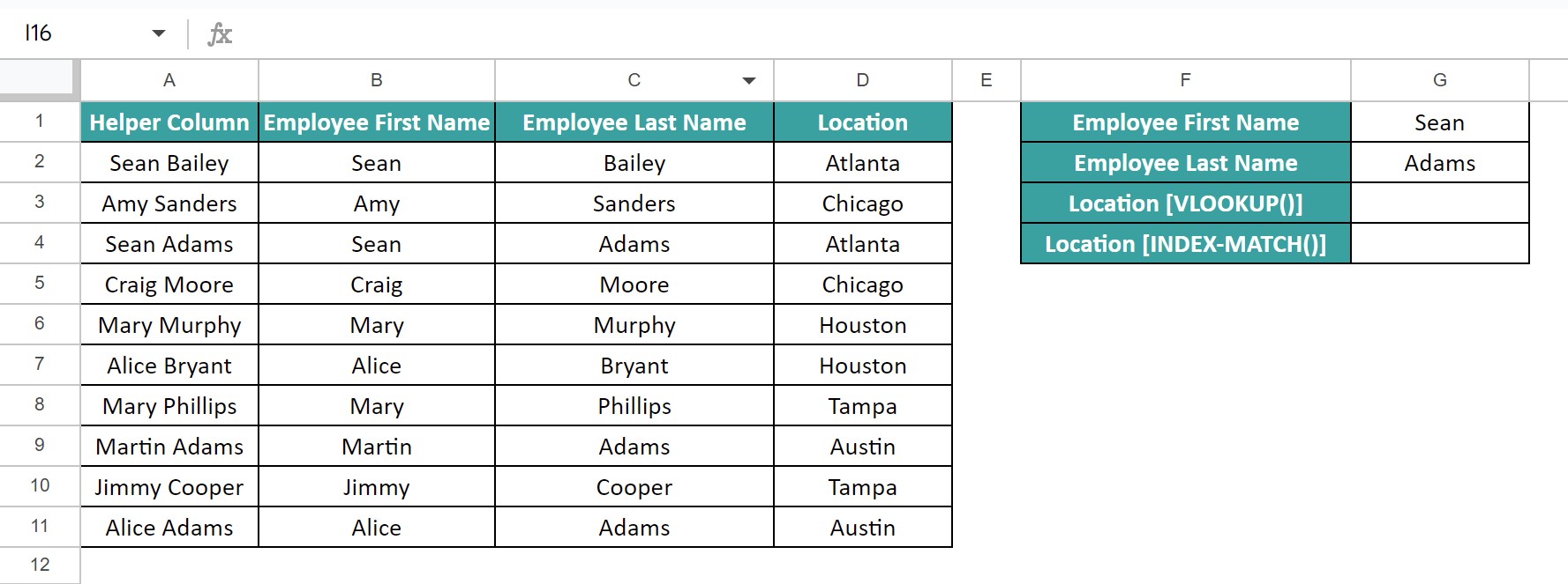
The aim is to update the specific employee location whose first and last names are in cells G1:G2.
We shall show how to secure the output using the multiple criteria-based VLOOKUP() in cell G3 and INDEX-MATCH() in cell G4.
Step 1: Select cell G3, enter the multiple criteria-based VLOOKUP(), and press Enter.
=VLOOKUP(G1&” “&G2,A2:D11,4,0)
Step 2: Select cell G4, enter the multiple criteria-based INDEX-MATCH(), and press Enter.
=INDEX(D2:D11,MATCH(G1&” “&G2,B2:B11&” “&C2:C11,0))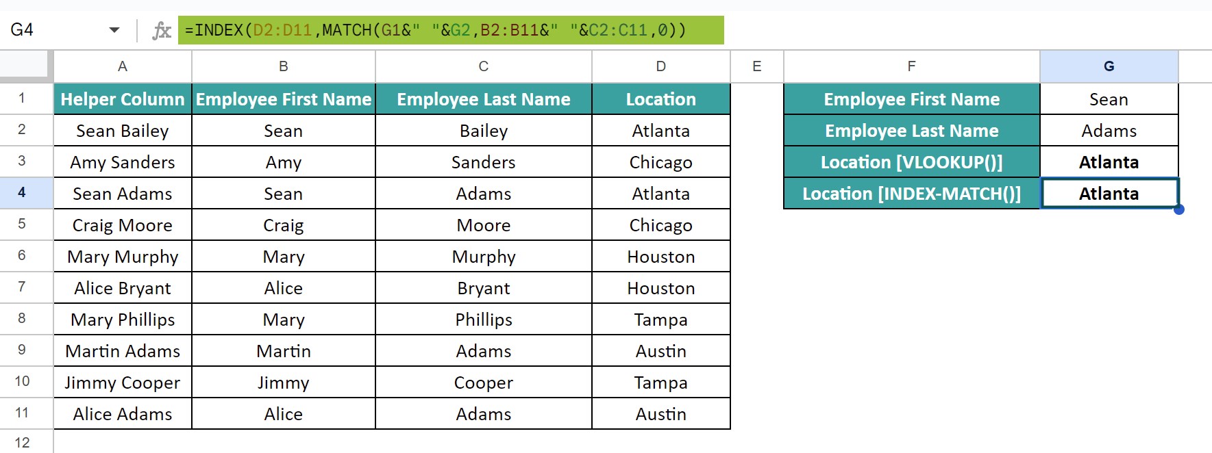
The VLOOKUP() based on multiple conditions requires a helper column, which shows the employees’ names concatenated to use as a unique search key. Also, the index argument value is hardcoded. If we modify the search range in the source dataset, the function might return an incorrect value.
In contrast, the INDEX-MATCH() based on multiple conditions does not involve a helper column and hardcoded column references. Instead, it uses dynamic column references.
We can have two or more criteria in INDEX MATCH in Google Sheets, which can go up to infinity.
Here, we can troubleshoot common issues with Google Sheets INDEX MATCH and multiple criteria using the following ways:
Ensure the formula syntax is correct, with the range references and conditions accurately specified.
Ensure that the data is formatted consistently throughout its range.
The source dataset should be accurate and without any missing data.
Ensure that the range references are correct and do not overlap.
Ensure that the conditions are appropriately formatted and that they apply to the concerned data range.
Use this INDEX MATCH Multiple Criteria In Google Sheets Template to follow along with the examples in this article.
Download Excel TemplateRecommended Articles
Continue with these related resources when you want the next practical step in this topic.
- LOOKUP in Google Sheets
- HLOOKUP In Google Sheets
- VLOOKUP Table Array In Google Sheets
- VLOOKUP True In Google Sheets
- INDEX MATCH Function In Google Sheets
Explore the full Google Sheets Lookup Functions guide or browse Google Sheets Resources.