
What Is Table Array In VLOOKUP Function?
The VLOOKUP table array is the second argument in the function. And it is a data range containing a minimum of two columns. The first column is where we can expect to find the lookup value. And a column on the right of the first column within the chosen data range will contain the value we require the VLOOKUP() to return in the target cell.
Users can specify the table array in the VLOOKUP() as a relative or absolute excel reference to a dataset in the same or different sheet. And thus, it makes the VLOOKUP function resourceful for fetching the corresponding data from within and outside the current sheet.
Use this VLOOKUP Table Array Template to follow along with the examples in this article.
Download Excel TemplateFor example, the first table lists items, their categories and quantities.
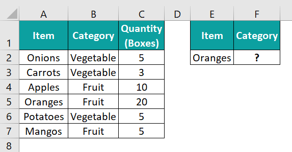
If the requirement is to update the category for the item cited in the second table based on the first table data. Then, we can use the VLOOKUP table array based on cell value concept to fetch the category data for the specified item, Oranges, in the target cell F2.
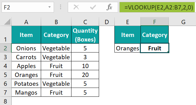
In the above VLOOKUP table array based on cell value example, the second argument in the VLOOKUP() is the table array, which is a relative reference to the cell range A2:B7.
It implies that the function in the target cell searches the lookup value, Oranges, in the cell range A2:B7 in the first column of the specified table array. And once it locates the first occurrence of the lookup value in column A, cell A5, it returns the data in the same row of the last column of the given table array, cell B5 value, Fruit.
And thus, the VLOOKUP() function return value in the target cell F2 gives the required category information of the item specified in cell E2.
Key Takeaways
- The VLOOKUP table array is the data range, with a minimum of two columns, which we supply as the second argument value to the function.
- Users can supply the appropriate table array to the VLOOKUP() when they must fill one table based on the data provided in another table in the same or different worksheet.
- We can supply the table_array argument value to the VLOOKUP() as a relative or absolute reference to a cell range in the same or different sheet or as a named range. Otherwise, we can keep it variable using the INDIRECT().
Examples
Check out the following examples that explain how to provide the table array value to the VLOOKUP() to use the function effectively.
Example #1
We shall see a VLOOKUP table array named range example.
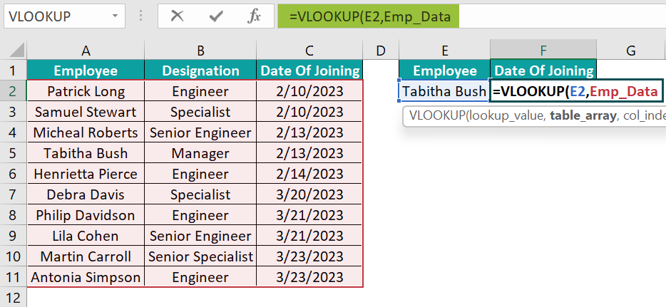
The first table lists employees, their designations and joining dates.
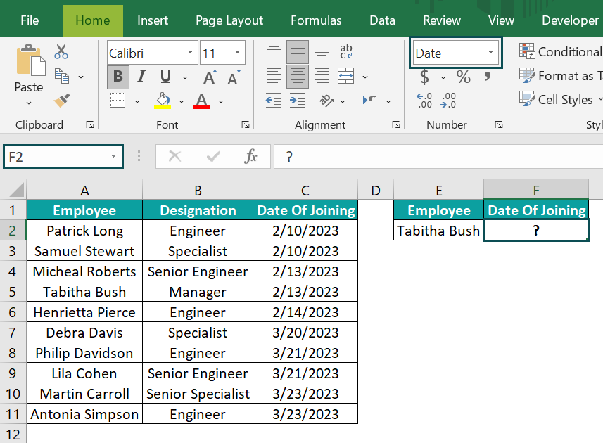
If the requirement is to update the joining date information for the employee specified in cell E2 in the second table based on the data in the first table. And assume the target cell is F2 with the data format set as Short Date in the Number Format option in the Home tab.
Then, we can use the named range in excel to make the VLOOKUP function return the required data in the target cell.
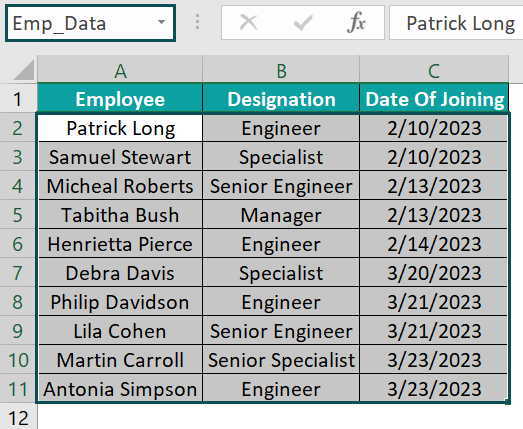
- Step 1: Select the cell range A2:C11 and type Emp_Data in the Name Box to create a named range.
[Alternatively, we can select the required cell range, click the Formulas tab and select the Define Name option.

The New Name window will open.
Otherwise, we can press Alt + M + M + D to access the New Name window.

Update the required name for the chosen cell range in the Name field in the New Name window.

And click OK to create the required named range.]
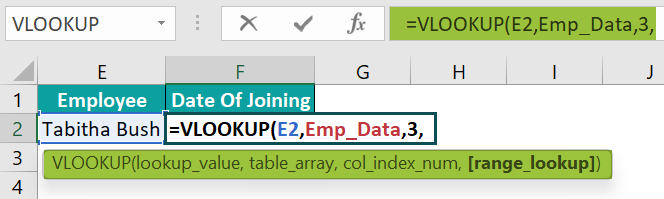
- Step 2: Choose the target cell F2 and start typing in the VLOOKUP(), as explained below.
=VLOOKUP(
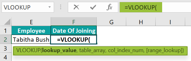
According to the VLOOKUP() syntax, we must enter the values for four arguments. While the first three arguments are compulsory, the fourth one is optional.
So, we will enter the first argument, lookup_value, as a reference to the cell containing the specific employee name in the second table, cell E2, followed by a comma.
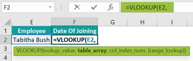
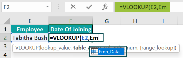
The second argument is table_array. And as we must get the required information based on the first table, we will provide the table_array value as the named range, Emp_Data. And for that, we can type “Em”, and Excel will show the named ranges starting with the specified phrase.
As we have only one named range starting with “Em”, we see one option, Emp_Data. Double-click it to choose it and enter a comma.
Next, we shall enter the third argument, col_index_num, as 3 since we need to display the joining date for the specified employee in the second table based on the source dataset. And the joining date data is available in the third column in the specified table_array named range.
And then enter a comma.
Next, once we enter a comma, Excel will show the options for an approximate and exact match as the last argument range_lookup value. And as we require an exact match, double-click the FALSE option to select it.
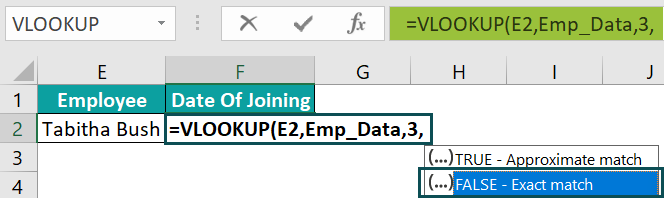

Finally, close the bracket.
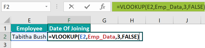
- Step 3: Press Enter to view the value the VLOOKUP() returns in the target cell.
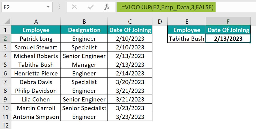
We created the source dataset as a named range, Emp_Data.
So, supplying it as the table array to the VLOOKUP() enables the function to search for the lookup value, Tabitha Bush, in the first column of the source data.
On the other hand, the argument col_index_num value is 3. It implies that the function must return the required value from the third column, column C, counted from the first column in the specified table array.
So, once the function finds its first occurrence in the first column, cell A5, it returns the data in the same row of the column specified by col_index_num, cell C5 value, 2/13/2023.
Example #2
The following illustration explains how to use the INDIRECT excel function as the table_array argument in the VLOOKUP() when the requirement is to look up the same value from multiple tables.
The two tables in the image below contain a list of students, their scores and their ranks in Mathematics and Science tests.

And the requirement is to update the ranks of a student, Ken Carpenter, in the two tests, based on the first two datasets. Assume the target cell range are D16:D17.
Then, here is how to use an INDIRECT()-based variable table array in the VLOOKUP() in the target cells to achieve the desired output.
Step 1: Choose the target cell D16, enter the VLOOKUP() containing the INDIRECT(), and press Enter.
=VLOOKUP(A16,INDIRECT(B16),3,0)

[ Alternatively, select cell D16 and choose the Formulas tab → Lookup & Reference function group → VLOOKUP function.

The Function Arguments window opens.

Next, we must update the argument values in the corresponding fields in the Function Arguments window.
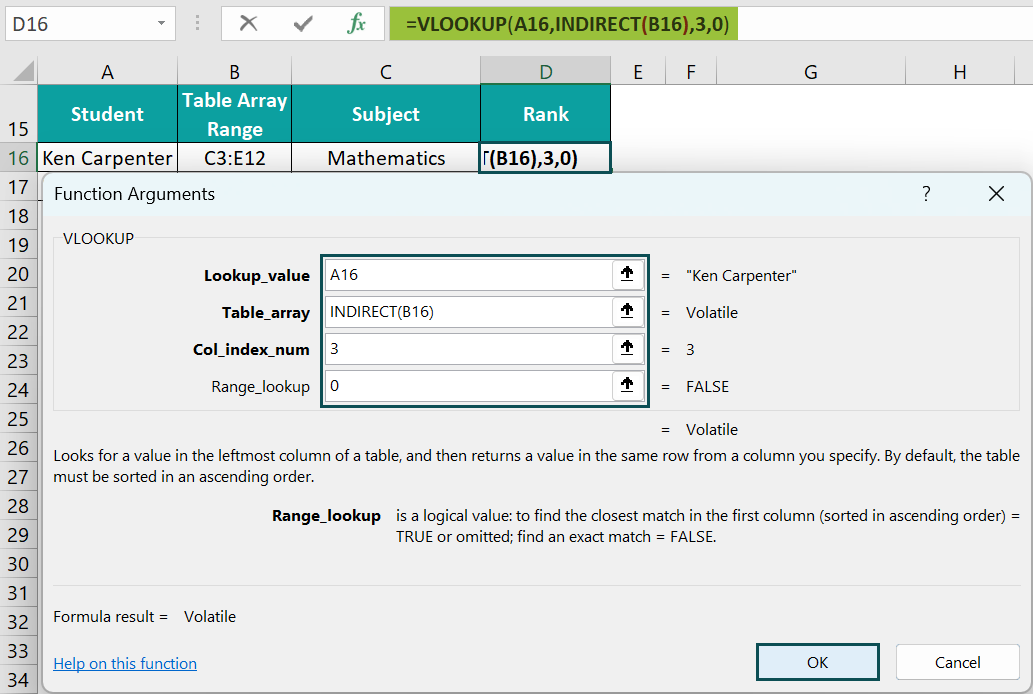
Finally, clicking OK will close the Function Arguments window. And we will get the required rank data in the target cell.]
- Step 3: Use the fill handle to enter the formula in cell D17.
=VLOOKUP(A17,INDIRECT(B17),3,0)

The VLOOKUP() in cell D16 accepts the reference to the cell containing the student name to lookup, cell A16. Next, the INDIRECT() accepts the reference to the cell containing the table array range to search for the lookup value, cell B16. And it returns the absolute reference of the specified cell range, $C$3:$E$12.
Further, as we require the rank data, the col_index_num argument value is 3, indicating column E of the first dataset. And, for an exact match, we set the last optional argument as 0, which interprets as FALSE.
And thus, based on the inputs, the VLOOKUP() searches for the specified student’s name in column C cells in the range, C3:C12. And as it locates the value in cell C9, it returns the value in cell E9, 8, as the student’s rank in the Mathematics test.
Furthermore, step 2 will set the first argument in the function as cell reference A17 and also update VLOOKUP table array argument value as INDIRECT(B17).
And thus, the function searches the lookup value in the new table array range $G$3:$G$12, which the INDIRECT() returns. It finds the lookup value in cell G7 and column I is the third column from the first column in the second dataset. So, the function returns the student’s rank in the Science test as the cell I7 value, 9.
Example #3
Let us see a VLOOKUP table array different sheet example.
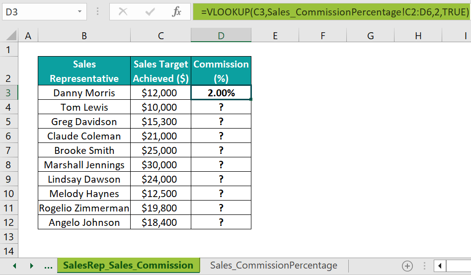
Consider we have two worksheets, SalesRep_Sales_Commission and Sales_CommissionPercentage.
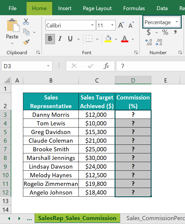

While the first one contains a list of sales representatives at a firm and their achieved sales targets, the second sheet contains the commissions one can earn for different sales figures.
And we must update the commission the sales representatives earned for their achieved sales targets in column D of the first sheet based on the second worksheet data. Also, the column D data format is Percentage in the Home tab → Number Format option.
Then, applying the VLOOKUP table array different sheet method, with an approximate match, will help us update the required values in the target cells.
However, ensure the data in the first column in the table array, referenced from the second sheet, must be in ascending order. Otherwise, the VLOOKUP() may return an incorrect value based on an approximate match.
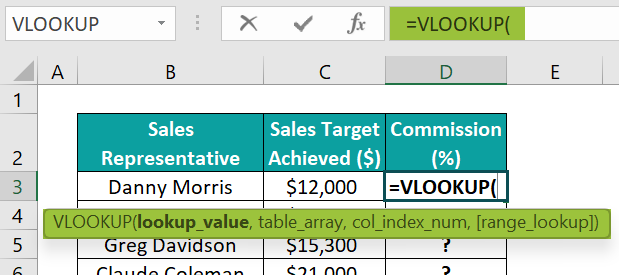
- Step 1: Choose the first target cell D3 and start typing in the VLOOKUP(), as explained below:
=VLOOKUP(
Next, we must look up the sales figure value provided in the first sheet in the second worksheet to find an approximate match for obtaining the required commission percentage.
The reason for finding an approximate match is that the commission percentages in the second sheet are for different sales value ranges. For example, if a sales representative achieved a sales target of $11,000. Then, as the value falls between $10,000 – $15,000, the commission percentage the representative earns will be 2%, based on the second sheet data.
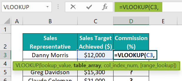
So, enter the lookup_value argument value, reference to cell C3, followed by a comma.
Next, click the second sheet tab and select the cell range C2:D6 to provide the table_array argument value, followed by a comma.
The above step will show the sheet name in the table_array argument as the reference is to a table array data in a different sheet.

And then, provide the col_index_num argument value as 2 since the commission percentage data is in the second column in the specified table array. And enter a comma.

And once we enter a comma, Excel will list the TRUE and FALSE options to choose the value for the last range_lookup argument. And as we aim to get an approximate match, we must double-click on the TRUE option to select it.


Finally, close the bracket.

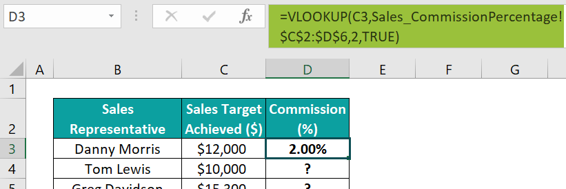
- Step 2: Press Enter to execute the formula in cell D3 in the first sheet.
However, using the fill handle to enter the above formula in the remaining target cells will update VLOOKUP table array range, as we provided a relative reference to the array range.
Thus, we must make the table array range reference absolute in the formula to keep it fixed. And for that, we must select the cell range in the table_array argument value in the cell D3 formula and press F4 to change the reference from relative to absolute.
- Step 3: Using the fill handle, update the formula in the remaining target cells.
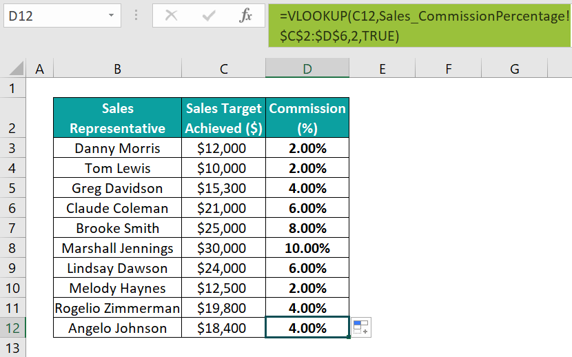
Let us see the cell D12 formula to understand how the table array reference from another sheet works.
The VLOOKUP() searches for the lookup value in cell C12 of the first sheet, $18,400, in the cell range C2:C6 in the second worksheet. And, as the lookup value is just over $15,000 and we chose the last argument value as TRUE, the VLOOKUP() finds an approximate match in cell C3. Thus, it returns the commission percentage in the same row in column D, the cell D3 value, 4.00%, as the output.
Important Things To Note
- Ensure the number of columns in the VLOOKUP table arrayequals at least the number supplied as the col_index_num argument value.
- If the requirement is to use the VLOOKUP() in contiguous cells, with the table array range being the same. Then, lock the table array when supplying it to the VLOOKUP() in the first cell.
- If the first column in the table array does not contain the lookup value, or the lookup value is below the lowest value in the first column in the lookup range. Then, the VLOOKUP() may not work for the specified table array.
Frequently Asked Questions (FAQs)
We can lock table array in VLOOKUP function by using the following methods:
• Absolute referencing the cell range when supplying it as the table_array argument value to the VLOOKUP().
• Supplying a named range as the table_array argument value to the VLOOKUP().
• Updating the VLOOKUP() in the worksheet and password-protecting the sheet.
The VLOOKUP table array is not working for the following reasons, which we shall see with an example.
The table below lists a set of products, their grades and costs.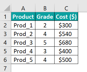
• The first column of the specified table array does not contain the lookup value.
For example, the requirement is to update the cost for the product specified in the second table based on the data provided in the first table. And assume the target cell is F1, with the data format set as Currency in the Home tab → Number Format option.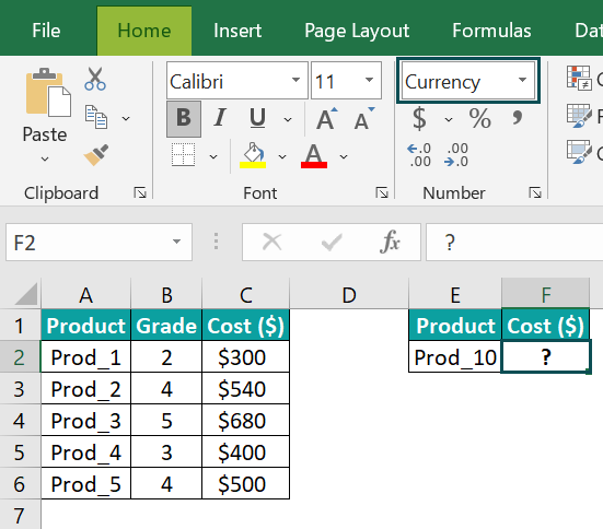
Then, we can use the VLOOKUP() in the target cell to obtain the required data, as shown below.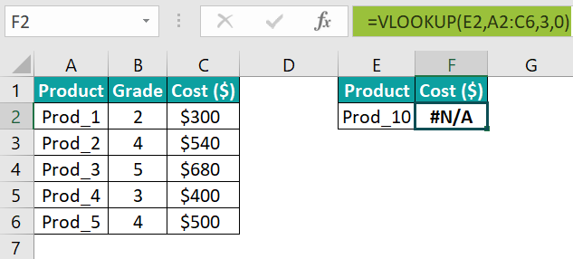
However, the function returns the #N/A error. And the reason is the lookup value in cell E1, Prod_10, is not present in the first column of the lookup range, specified as the table_array argument value.
• The lookup value is below the least value in the table array’s first column.
For example, the requirement is to update the cost of a Grade 1 product in cell F6 in the third table based on the data in the first table. And the data format of cell F6 is Currency.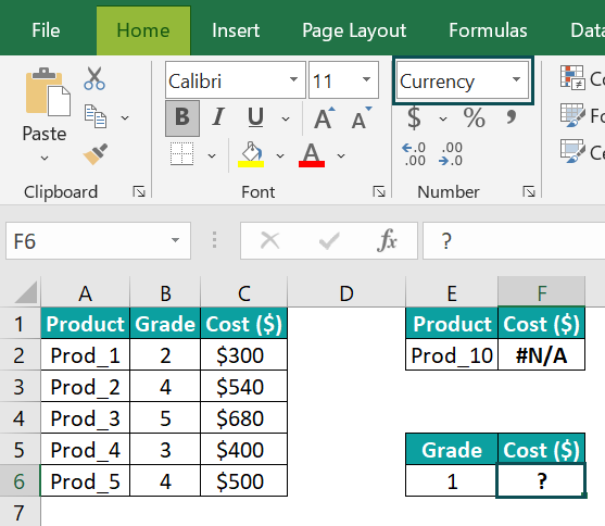
Then, using the VLOOKUP() in the target cell will fetch us the required data. However, whether it is an approximate or exact match, the function returns the #N/A error.
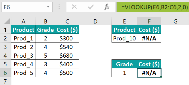
The reason is that the lookup value, 1, given in cell E6, is below the lowest value in the first column of the specified table array, 2.
• The table array is not locked.
For example, the requirement is to update the cost of the two products specified in the fourth table based on the first table data. And assume the target cell range is F10:F11, with the data format set as Currency.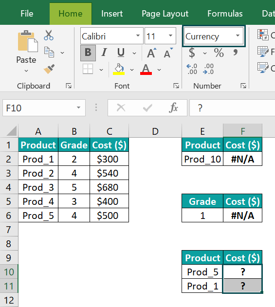
Then, using the VLOOKUP() in the target cells will fetch the required output. And for that, we can enter the VLOOKUP() in cell F10 and then drag the fill handle downwards to update the formula in cell F11.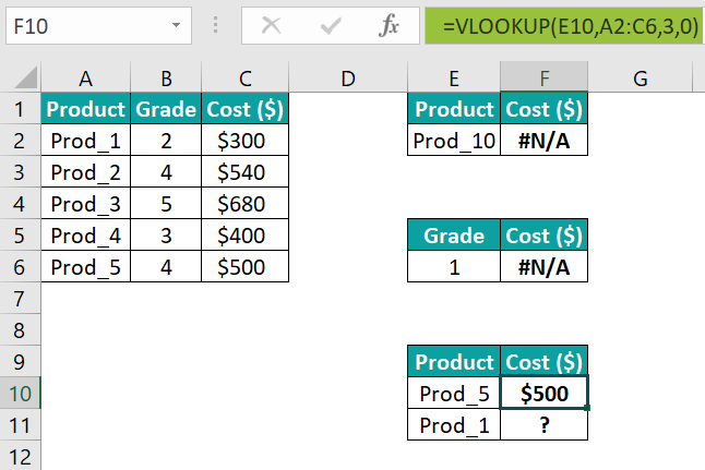
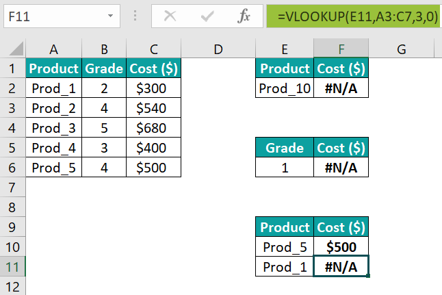
While the VLOOKUP() returns the correct value in the first target cell F10, its output is the #N/A error in the second target cell F11.
Since we did not use the absolute reference to the table array range, the table array range changed when we used the fill handle to update the formula in cell F11. And as the lookup value is not in the updated lookup range, the function returns the error.
The shortcut for table array in VLOOKUP function is to click the first cell in the lookup range and then press the keys Ctrl + Shift + ↓ + →.
The shortcut will select the cells down the first column until an empty cell. And then, it will choose the cells in the same rows, as chosen in the first column, in the columns on the right of the first column till the first empty column.
Use this VLOOKUP Table Array Template to follow along with the examples in this article.
Download Excel Template