Break-Even Analysis In Excel

What Is Break-Even Analysis Excel Function?

The break-even analysis in Excel involves determining the point at which the total cost incurred equals the total earnings. Graphically, the break-even point is the coordinate where the total revenue and total expense curves cut each other.

Users can use the break-even analysis Excel function when estimating the pricing of items to ensure the revenue exceeds the costs.

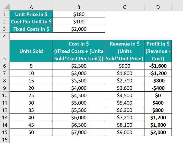
For example, the first table contains the unit price, cost per unit, and fixed costs details.

And, based on the first table data and the units sold data in the second table, we populate columns B:D in the second table. We can refer to the column headings in the second table for the applied formulas in the respective columns.

The above table shows the break-even point based on units sold, which occurs when the units sold are 25. It is where the costs and revenue are equal.

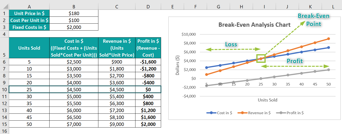
Further, the below plot helps perform the break-even analysis in Excel visually.

The above break-even analysis plot corroborates our findings based on the profit data in the table. And the cost and revenue curves meet when the units sold are 25 at a unit price of $180.

Thus, the inference is that if we wish to achieve the break-even point, we must sell 25 units, and selling more than 25 units will earn us profits.

How To Do Break-Even Analysis?

We can perform the break-even analysis in Excel using the following methods:

• Goal Seek feature
• Break-Even table
• Break even analysis formula in Excel

Let us see each method with an example.

Example #1 – Using Goal Seek

The following example explains how to conduct a break-even analysis in Excel using the Goal Seek feature from the Data tab.

Consider the situation where we plan to sell a product. And assume that we are aware of the variable cost per unit and the overall fixed costs.

Suppose we estimate the feasible sales volumes (Unit Sold), and based on the prediction, we fix the product price (Unit Price).

So, here is how to use the Goal Seek feature to determine the break-even unit price in cell D3, such that the profit is $0.

• Step 1: First, select cell D5, enter the formula to find the unit price and unit sold product, and then, press Enter. It will give the total revenue.

=D3*D4

• Step 2: Next, select cell D7, enter the below formula to find the product of the unit sold and cost per unit, and then, press Enter. It will give the variable costs.

=D4*D6

• Step 3: Then, select cell D9, enter the below formula to deduct the variable and fixed costs from the revenue, and press Enter. It will give the profit gained.

=D5-D7-D8

• Step 4: Now, click Data → What-If Analysis → Goal Seek option to open the Goal Seek window.

• Step 5: Update the three fields in the Goal Seek window, as shown below:

As the target profit value is $0, the first and second fields are the absolute reference in excel to cell D9 containing the profit value and 0, respectively.

Further, the requirement is to achieve $0 profit by changing the unit price. So, the last field is the absolute reference to cell D3, containing the unit price.

• Step 6: Once we click OK, the Goal Seek Status window will open.

And clicking OK will close the Goal Seek Status window.

Thus, the final table will appear as shown below. Also, it includes a column showing the formulas used in column D cells.

The unit price changes from $30 to $34 ($33.75, to be precise), and the total profit becomes $0. Hence, if we estimate the sales volume as 80, the unit price should equal or exceed $34. Otherwise, we will face losses.

We may set the above table as a break even analysis in Excel template when we need to determine the break-even point based on the unit price of a product.

Example #2 – Using A Break-Even Table

Let us see an example of a break-even analysis in Excel using a break-even table.

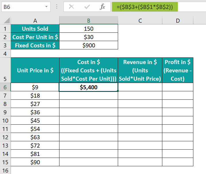
The first table contains a product’s details about units sold, cost per unit, and fixed costs.

Suppose the second table contains unit prices. And based on the given details, we must calculate the total costs, revenue, and profit data to obtain the break-even price in the second table.

Then, we can apply the below-shown formulas and use the two tables as a break even analysis in Excel template to achieve the break-even point based on unit price.

• Step 1: Select cell B6, enter the below formula to get the total costs for the specified unit price, and press Enter.

=($B$3+($B$1*$B$2))

• Step 2: Select cell C6, enter the formula to determine the revenue as the product of units sold and unit price, and press Enter.

=$B$1*A6

• Step 3: Select cell D6, enter the formula to calculate the profit as the difference between revenue and cost, and press Enter.

=C6-B6

• Step 4: Select cells in the range B6:D6, and using the fill handle in excel, enter the formulas in the cell range B7:D15.

The above table shows that the revenue equals the total cost when the unit price is $36, which becomes the break-even price.

Let us show the costs, revenue, and profit curves in a break-even chart to confirm the break-even price.

• Step 5: Select the cell range B5:D15 and select Insert → Line or Area Chart → Line with Markers chart.

Next, we shall modify the legend series for better understanding.

• Step 6: Right-click the chart area and pick the Select Data option from the context menu.

• Step 7: The Select Data Source window will open. Click on the first entry in the Legends Entries field and click Edit.

• Step 8: The Edit Series window will open, where we can update the Series name to show the corresponding legend as per the requirement.

Click OK to go back to the Select Data Source window.

• Step 9: Repeat steps 7 and 8 to update the remaining legend series.

Next, we require the unit price on the X-axis to verify the break-even price.

• Step 10: Click the Revenue in $ legend series and click Edit in the Horizontal Axis Labels field.

• Step 11: The Axis Labels window opens up. Enter the unit price cell range A6:A15 in the required field and click OK.

And clicking OK will close the Select Data Source window.

• Step 12: Click the chart area to enable the Chart Elements option (‘+’ icon) and check the Axis Titles box.

• Step 13: Update the chart title and axis titles using the respective elements in the chart area to get the below plot.

Initially, the revenue curve is below the cost curve, implying losses, with the profits being negative. Then, when the unit price is $36, the revenue and cost curves intersect, indicating a no-profit and no-loss scenario.

And after the break-even point (highlighted in the above image), the revenue curve improves and crosses the cost curve. It indicates that for unit prices above $36, the unit volume of 100 sold yields profits.

Example #3 – Using Break-Even Analysis Formula

Using formulas, we can determine the break-even point by parameters such as total sales, units, and unit price. However, we must apply the appropriate formula to perform an accurate break-even analysis.

For example, assume a product is sold at a firm. And we calculated the fixed costs at the firm as $50,000. On the other hand, the variable expense incurred while producing the product is $5 per unit, and we sell the product at a unit sales price of $15.

The requirement is to determine the break-even point of the firm by unit and display the result in cell C7.

Then, we can apply the below break even analysis formula in Excel cell C7 to achieve the required information.

Break Even Unit = Total Fixed Costs / (Unit Sales Price – Variable Cost Per Unit)

• Step 1: Select the target cell C7, enter the below formula, and press Enter.

=C5/(C3-C4)

Thus, for the specified total fixed and variable costs and unit sales price of the product, the firm must sell 5,000 units of the product to recover expenses.

Example #4 – Creating A Break Even Analysis Calculator

Suppose we set the profit as $0. And we pre-forecast the units sold, the cost per unit, and the fixed costs.

Then, we can create a break even analysis calculator Excel to obtain the required break-even point by unit price.

For example, a calculator with the required formulas below will help us conveniently perform the break-even analysis in Excel.

• Formulas Explanation
  • Unit Price: Divide the fixed costs by units sold and then add the cost per unit to the result.
  • Revenue: Find the product of unit price and units sold.
  • Variable Costs: Find the product of units sold and cost per unit.

• Step 1: Enter the required units sold, cost per unit, fixed costs, and profit in cells C4, C6, and C8:C9, respectively.

Once we update the above mentioned data in the specified cells, the formulas in cells C3, C5, and C7 update the unit price, revenue, and variable costs.

So, we can now modify the pre-estimated values in the calculator to evaluate the unit price automatically and perform the required break-even analysis easily.

Important Things To Note

• Ensure the source data contains valid numbers to perform the break-even analysis in Excel correctly.
• When creating the break-even chart for analysis, update the X-axis as the data series based on which you intend to determine the break-even point.
• We can perform a break-even analysis based on different parameters, such as units and unit price. So, ensure we use the appropriate break-even formula to conduct the analysis correctly.

Frequently Asked Questions (FAQs)

Download Template

This article must be helpful to understand the Break-Even Analysis In Excel, with its formula and examples. You can download the template here to use it instantly.

Recommended Articles

This has been a guide to Break-Even Analysis In Excel. Here, we explain methods to perform break-even analysis, with examples & downloadable excel template. You can learn more from the following articles –

• PRICE Function In Excel
• CLEAN Excel Function
• Alternatives to VLOOKUP In Excel