
What is BYCOL in Google Sheets?
The BYCOL function groups an array by columns by applying a LAMBDA function to each column. BYCOL in Google Sheets operates on a range or array and returns an array of a row, that is created by grouping each column to a single value. This function is beneficial when you wish to apply the LAMBDA function by columns and show the result of each calculation in a row. Thus, one need not copy and paste a formula to all cells in which one must show the results of the calculation.
As an example, let’s say we have the following values in A1:C4. Now to calculate the sum of each column, we use the following formula:
Use this BYCOL in Google Sheets Template to follow along with the examples in this article.
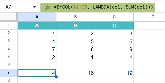
Download Excel Template=BYCOL(A2:C5, LAMBDA(col, SUM(col))).
(Here, col is just a placeholder variable used in the LAMBDA function. Representing each column.). The formula returns the following result, [14, 16, 19] because they are the sum of the values in each column.
Key Takeaways
- BYCOL in Google Sheets applies a custom function to each column in a given range, returning one result per column.
- The syntax of the function is: =BYCOL(array_or_range, LAMBDA(column, calculation))
It must always be used with a LAMBDA function that defines how to process each column. - You can combine BYCOL with functions like SUM, AVERAGE, COUNTIF, MAX, and logical expressions (IF, SWITCH).
- BYCOL is used for applications like analyzing test scores, survey data, and sales metrics.
Syntax
The BYCOL formula in Google Sheets is as follows:
=BYCOL(array_or_range, lambda)
- Array_or_range: This array or range is used as the input to the LAMBDA function.
- Lambda: we define this function as LAMBDA(column, average(column)) with one argument and “formula_expression”. The argument given corresponds to a series of values in a column. Named functions can also be used.
How To Use BYCOL Function in Google Sheets?
If you’re left wondering on where BYCOL in Google Sheets can be used, let us give you a simple example with an explanation on how it works column by column. The function can be entered in Google Sheets in two ways:
- Manually enter BYCOL
- Enter through the Google top menu
It is especially useful when working with sales data or performance metrics, where one has to summarize each column individually.
Let’s explore how to use it with a simple example.
Entering BYCOL Manually
In this example we have a few values in a range.
Step 1: To enter the function manually, we must supply the range and also the custom LAMBDA function.
Enter the details in a Google Sheet. This is the data from which we’ll calculate the sum of each column.

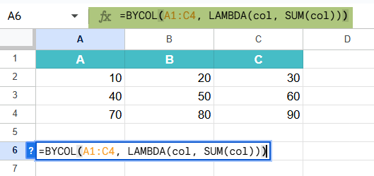
Step 2: Click on an empty cell (here we select cell A6) and type the following formula manually.
- First, enter the = sign followed by the function name with open parentheses.
- Enter the required range, followed by LAMBDA and the arguments as shown below.
- Close the parentheses for both LAMBDA and BYCOL.
=BYCOL(A1:C4, LAMBDA(col, SUM(col)))
This formula calculates the sum of each column in the range A1:C3.
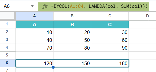
Step 3: Press Enter. You will now see the result as an array. Thus, each element of the resultant array shows the sum of the corresponding column’s values. [120, 150, 180]
Insert Through Google Menu Bar
- Go to “Insert” → “Function” → “Array” → “BYCOL”.
- Select a range to which you want to apply the LAMBDA by columns.
- Enter a LAMBDA function with a placeholder and logic.
- Press the Enter key.
Examples
In many real-life scenarios we must find the highest value or average in each column of a data set. It could include scenarios such as sales data and test score. These and other uses are what define the BYCOL function which we will study with some interesting BYCOL in Google Sheets examples below.
Example #1 – Finding Maximum Values
In this example, there is a business tracking weekly sales for three different products over a month. The sales team wants to find the maximum weekly sales achieved for each product. For this, they can use the BYCOL function to automate this calculation within a single formula.
Step 1: Input the data as shown below in a new sheet.
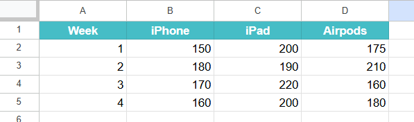
Step 2: Use the BYCOL formula to calculate the maximum values for each product as follows:
=BYCOL(B2:D5, LAMBDA(col, MAX(col)))
Explanation:
A2:C5 is the range of the sales data.
LAMBDA(col, MAX(col)) is used to apply the MAX function to each column individually.

Step 3: Press Enter. Google Sheets will return an array with three values. Each number corresponds to the maximum value found in each column.
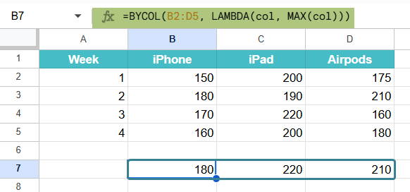
The output shows the highest weekly sales for each of the products. This can help the business identify which week had peak performance for each product and make decisions such as planning future inventory.
Thus, the BYCOL function can be efficiently used to compute column-based summaries like maximum values. This is useful for performance monitoring and trend analysis.
Example #2 – Calculating Column Averages
In scenarios such as when analyzing academic grades or sales trends, we will wish to find the average performance across different categories. In this example, let us use BYCOL to calculate the average score for each test. This not only saves time but also ensures consistency and accuracy in the calculations.
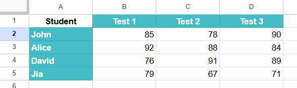
Step 1: Enter the details such as inputting test scores of three students for different tests. This is the structure in which we enter the data as it helps us evaluate the average score for each test across all students.
Step 2: Apply the BYCOL formula with AVERAGE to compute averages for each of the columns as follows:
=BYCOL(B2:D5, LAMBDA(col, AVERAGE(col)))
Explanation:
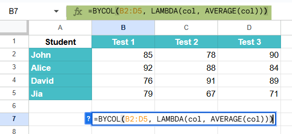
- B2:D5 is the data range containing the test scores.
- The LAMBDA(col, AVERAGE(col)) function takes each column and calculates its average.
Step 3: Press Enter. You get an array with the average score for each test. This gives you an instant overview of how the class performed on each test.
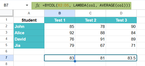
This helps the teacher spot which test had the highest or lowest average score. It can help adjust future teaching strategies.
By using BYCOL with AVERAGE, one can quickly calculate averages for each column in the dataset and is helpful for summarizing performance data.
Example #3 – COUNTIF for Each Column
In this example, a teacher wants to calculate how many students scored above 85 in each test. It is a hassle to manually filter the date or time consuming to apply individual formulas for each column. Hence, we can use the BYCOL function with LAMBDA and COUNTIF to dynamically compute the count for each test.
Step 1: Enter all the details in a sheet. Here, we have the test scores for four students across 4 different tests. We must evaluate how many students scored greater than 85 in each test.

Step 2: Enter the BYCOL formula with COUNTIF logic as shown below.
=BYCOL(B2:E5, LAMBDA(col, COUNTIF(col, “>85”)))
Explanation:
- B2:E5 is the data range for all the scores.
- LAMBDA(col, COUNTIF(col, “>85”)) counts how many values in each column are greater than 85.

Step 3: Press Enter. The formula will return an array with the number of students who scored above 85 in each test. This lets you immediately assess which test had more high performers.
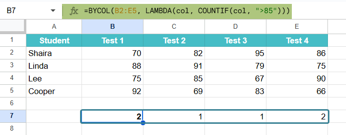
- Test 1: 2 students scored >85 (88, 92)
- Test 2: 1 student scored >85 (91)
- Test 3: 1 student scored >85 (95)
- Test 4: 2 students scored >85 (86, 90)
Thus, by using BYCOL with COUNTIF, we can identify how many values in each column meet a certain condition. It helps the teacher identify high-performing tests at a glance.
Important Things to Note
- If one gives an invalid LAMBDA function or an incorrect number of parameters, the formula returns a #VALUE! error.
- The output of BYCOL in Google Sheets is an array containing one result for each column. Thus, it will automatically spill across cells to the right.
- Not providing a LAMBDA function returns a #CALC error.
- This function is especially useful for large datasets because it eliminates the need to write separate formulas for each column. The single function is enough for the entire array.
Frequently Asked Questions (FAQs)
In Google Sheets, we have two similar functions: BYCOL and BYROW.
The main difference is in how the function processes data.
BYCOL applies a formula to each column, whereas BYROW applies it to each row.
For scenarios such as sales, if we are analyzing sales numbers across several salespersons (rows) and multiple months (columns), BYCOL gives you summaries for each month. For the same table, if we use BYROW, it will give you summaries for each salesperson.
LAMBDA is used in both functions to define the operation, but their orientation differs.
BYCOL works well with conditional functions like COUNTIF, AVERAGEIF, and also with nested IF statements inside LAMBDA. For instance,
=BYCOL(A1:C5, LAMBDA(col, AVERAGEIF(col, “>70”))) calculates the average of values greater than 70 in each column from range A1 to C5.
Thus, BYCOL is highly flexible for data filtering and conditional analysis without any need for helper columns. It works best when paired with aggregate functions.
BYCOL requires a LAMBDA function because it processes each column independently. It also needs a function like SUM or AVERAGE to tell it what to do with each column. The LAMBDA is used to define a variable (commonly col) that represents one column at a time. Here, we specify what operation should be done to a column. For example,
=BYCOL(A1:C5, LAMBDA(col, MAX(col)))
Here, LAMBDA(col, MAX(col)) finds the maximum value of each column in the range A1:C5.
Use this BYCOL in Google Sheets Template to follow along with the examples in this article.
Download Excel Template