What Is Checkbox In Excel?
Checkbox is an object which can take a tick mark as an input. A checkbox is a little square object which allows the user to select or deselect action items. A checkbox is often called a checkmark box or select box.
When we ask people to select something traditionally, we give them a blank space to write YES or NO. However, to make things more professional, we can use checkbox in excel.
There are 2 types of checkbox in Excel. They are:
- Form Control Checkbox: It is the basic version of the checkbox in excel. We cannot edit any of the properties of the checkbox in the form control checkbox.
- ActiveX Control Checkbox: It is the advanced version and also supports VBA macro coding. In this version of the checkbox, we can change the properties of the checkbox, and this is versatile and flexible.
Let us understand the steps used to create checkbox in excel with the following example.
Step 1: First, go to the Developer tab. Click on Insert and select the checkbox option from the Form Controls category.

We can see a checkbox option in the worksheet, as shown in the image below.

Step 2: Next, right-click on the checkbox and select the Format Control… option.

Step 3: The Format Control window appears. In the Cell link: box, select any cell. For our example, let us select cell A4.

Step 4: Then, click OK.
Now, we can see the value TRUE in cell A4 whenever we click on the checkbox in excel.

Likewise, we can use checkbox in excel to present our worksheets better.
Table of contents
Key Takeaways
- The checkbox in Excel is the tiny box used to select or deselect action items in Excel. It is also called select box.
- A checkbox returns TRUE if checked, or it will return FALSE.
- Creating interactive charts is possible with a checkbox in Excel.
- Conditional formatting is applied to the checklist based on the checklist selection.
- We can create checkbox in Excel using Developer -> Insert -> Checkbox. However, users can use checkbox in excel without the developer tab by changing the font name and character code in the Symbols category.
Enable The Developer Tab
However, we may not see the Developer tab in the Excel ribbon because by default, the function is disabled.

Hence, we need to enable it to use checkbox in excel.
The following steps are used to enable Developer tab in Excel.
Step 1: To begin with, go to the File tab.

Step 2: Next, click on Options.

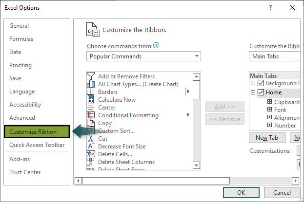
Step 3: The Excel Options window pops up. Then, click on the Customize Ribbon option.

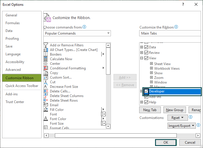
Step 4: Next, select the Excel Developer tab under Main Tabs.

Step 5: Click OK. Now we will be able to see Developer tab.

Now, we can use options such as the checkbox in excel, which are available under the Developer tab.
How To Insert A Checkbox In Excel?
Inserting Checkbox in excel is quite simple. Let us learn how to insert checkbox in excel with the following steps.
- Go to the Developer
- Click on the drop-down list of the Insert
- Select the Checkbox option

- Now, draw the checkbox on the worksheet.

Once the checkbox is inserted into the worksheet, we need to link this checkbox to any of the cells in the worksheet.
Right-click on the inserted checkbox and click on Format Control.

The Format Control window opens up.
Value: Choose the Checked option. It will make the checkbox marked whenever the workbook opens up.
Cell Link: Give any of the cell’s references in this box. We can choose the cell or enter the cell address manually.
Click OK after making all the changes as shown in the above picture.
Now, we have linked the checkbox to cell A10. When we select the checkbox, we will get the TRUE value in cell A10. We will get the value as FALSE if the checkbox is not selected.


Checkbox In Excel Examples
Example #1: Create A Check List With Conditional Formatting
By using the checkbox, we can create some interactive checklists. Assume that we are traveling and we need to prepare a checklist and want to make sure we track the preparation without missing anything.
Following is the traditional checklist for traveling.

When the line items are completed, we need to check and highlight them. Follow the below steps to add checkbox in excel and apply conditional formatting.
Step 1: Go to the Developer tab, and click on the Insert option. Next, select the Checkbox in excel option.

Step 2: Now, draw the checkbox in the worksheet.

Step 3: Right-click the inserted checkbox and select the Format Control… option.

Step 4: In the Format Control window, choose the Checked option and select the excel cell reference as cell C2 in the Cell link: box.

Now, when we select the checkbox, we will see the TRUE value in cell C2, or else we will see the FALSE value.
Step 5: Again, right-click the checkbox and choose Edit Text.

Step 6: Remove the text and make it blank.

Step 7: Adjust the checkbox to the middle of the cell.

Step 8: We also need to do the same for the remaining cells.
Since inserting them one by one is time-consuming, we can use the AutoFill excel option.

Step 9: As of now, all the checkboxes are linked to cell C2.
We need to change the linked cell to each checkbox’s cells.

As we can see, cell B3’s checkbox is linked with cell C3. Similarly, we need to do it for all the remaining cells.

Now, based on the checkbox selection, we should see either TRUE or FALSE in all the linked cells.
Whenever we complete the task, we will tick the checkbox and know that the particular task is completed.
However, to make it more appealing, we can apply conditional formatting to highlight the completed tasks based on the selection from the checkbox.
Apply Conditional Formatting
Step 1: Select the cells from A2:A9.

Step 2: Go to the Home tab, click on the conditional formatting drop-down option and choose New Rule… option.

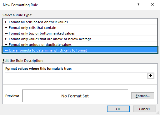
Step 3: The New Formatting Rule window opens up. Choose Use a formula to determine which cells to format option.

Step 4: In Format values where this formula is true: box, enter the following formula.
=$C2=TRUE

Formula Explanation: Whenever we select the checkbox, we will get the TRUE value in column C. So, if the cell value is TRUE, we need to format the selected cells.
Step 5: Click on the Format option in the same window.

Step 6: In the Format Cells window, choose Fill and select the color that we want to highlight the checklist.

Step 7: After choosing the fill color, click on the Font tab and select the Strike through option.

Step 8: Click OK in the next two windows, and conditional formatting will be ready.

Whenever we select the checkbox, conditional formatting will fill that checklist with chosen color and strike through the text.
Now, hide excel column C to make it look clean.
Example #2: Create Dynamic Chart Using Checkbox
When we have multiple datasets, it is unnecessary to show every data point in our visualization. By using checkbox in excel, we can allow the user to choose the data points they want to see.
We have the following data in Excel.

To create an interactive chart, we need to insert two checkboxes.

Change the text of the two checkboxes to 2019 and 2020.

For the 2019 checkbox, give a cell reference of G1.

For the 2020 checkbox, give a cell reference of I1.

Using these checkboxes activities, we need to create another data table like the following one.

When we select the 2019 checkbox, we get the values from the main table; otherwise, we will get an NA error.
Similarly, apply the formula for the year 2020 as well.

So, this formula will retrieve the values for the year 2020 if the checkbox is marked; otherwise, an NA error occurs.
For the year 2021, we will keep the static values by giving just references for the main table cells.

Select the newly created table range from F2:I6.
Go to the Insert tab and insert an excel combo chart, as shown in the following image.

The 2019 and 2020 numbers are converted to a line chart to compare the values with 2021.
If we want to compare the year 2020, then uncheck the 2019 checkbox. We will see only 2020 values in the chart.

In this way, we can create interactive charts using checkboxes.
How To Delete A Checkbox In Excel?
Once the checkboxes are inserted in an Excel worksheet, we can easily select a single checkbox by selecting and hitting the delete button.
To delete multiple checkboxes, we need to hold the control key and select the checkbox one by one.
However, this is time consuming. For a quick way, first, delete the checkboxes and then follow the steps listed here:
Step 1: First, go to the Home tab.
Step 2: Under the Editing group, click the Find and Select drop-down option and select the Selection Pane… option.

Step 3: The selection pane appears on the right of the Excel worksheet.

As we can see, we have checkbox names listed here.
Special Note: Checkbox caption and Checkbox names are two different things. For instance, take a look at the following image.

We have five checkboxes. Whatever we are seeing in the checkboxes in the caption and whatever we see on the selection pane are checkbox names.
For instance, there are 5 checkboxes. If we click on Checkbox 3 from the selection pane, it will select the inserted 3rd checkbox.

As we can see, excel has selected the position of the 5th checkbox in the worksheet even though in the selection pane, the selected option is checkbox 3.
So, the selection pane chooses the particular checkbox in the worksheet irrespective of its position in the worksheet.
To select all the checkboxes in the selection pane, press Ctrl + A to select all the checkboxes in one click.

Press the Delete key to delete checkboxes in one click.
How To Insert Checkbox In Excel Without Developer Tab?
We can insert Checkbox in Excel without the Developer tab as well. The following steps are used to insert checkbox in excel without the Developer tab.
Step 1: First, go to the Insert tab, click the Symbols drop-down and choose the symbol from the list.

Step 2: The Symbol window pops up. Now, change the font to Wingdings.

Step 3: Next, change the Character code: to 252.

Step 4: Next, choose the checkbox symbol from the symbol list.

Step 5: Click on the Insert option to create checkbox in excel.
Important Things To Note
- A checkbox is an object that can be movable in Excel.
- While using Checkbox option in the Form Control category, we cannot change the properties of the checkbox.
- The checkbox requires a cell reference to interact with the cell.
- Also, we can create checkbox in excel even without the Developer tab. To insert, we need to change the font to wingdings in the Symbols category.
- To select multiple checkboxes, we need to hold the control key and continue on the checkboxes that we need to select.

Frequently Asked Questions (FAQs)
To insert multiple checkboxes, first, we need to insert one checkbox.
Then, adjust the checkbox to fit inside the cell.
Now, select the checkbox option and drag it to the other cells using the fill handle.
We can insert multiple checkboxes in excel with ease.
Checkbox in Excel is available under the Developer tab.
To insert a yes, or no checkbox, first, we need to insert the Group Box.
Once the group box is inserted, we can see a group box, as shown in the following image.
Next, we need to insert Option Button twice.
Next, rename the caption to Yes and No.
If the checkbox is inserted from the ActiveX Control, we cannot delete the checkbox directly.
To delete, click on the Design Mode under the Developer tab.
Now we can select any checkboxes inserted from the ActiveX Control and delete them.
Download Template
This article must help understand Checkbox in Excel with its formula and examples. You can download the template here to use it instantly.
Recommended Articles
This has been a guide to Checkbox in Excel. Here we discuss how to insert, edit, delete checkboxes with examples and downloadable excel template. You can learn more from the following articles –

Leave a Reply