
Chi-Square Test In Excel
The Chi-Square Test in Excel is a distribution-free test that follows a statistical procedure for comparing and finding the relationship between categorical variables. We can derive a set of expected results using the given data, which is called the observed data, and then evaluate if there exists a relation between the observed and the expected results.
For example, the below table shows the observed orders delivered frequencies of two branch offices. And row 9 shows each column’s sum, and column D shows each row’s sum.

Consider we take a random sample of 1000 orders delivered by Branch Offices 1 and 2 together.
Use this Chi-Square Test In Excel Template to follow along with the examples in this article.
Download Excel TemplateAnd the null and alternative hypotheses (H0 and H1) are that the number of orders delivered does not depend and depends on the day of the week, respectively. Assume the significance threshold is 0.05.
We must conclude whether to accept or reject the null hypothesis (H0), and then calculate the Chi-Square Test in Excel as depicted below to make the decision.


As the first step in the above example, we must calculate the expected orders delivered frequencies for the two branch offices. Next, calculate the Chi-Square Test in Excel data points (refer to the third table), and adding the values will give us the Chi-Square (χ2), 21.34549532. And then using the CHISQ.INV.RT(), calculate the Chi-Square critical value, 9.487729037. Also, as the source data contains five rows and two columns of data (cell range B4:C8), the degree of freedom is 4.
Finally, apply the CHISQ.TEST() to determine the p-value, 0.000270432.
Thus, the above calculations show the χ2 statistic for the given data is 21.34549532, with 4 degrees of freedom. And the Chi-Square statistic, 21.34549532, exceeds the determined critical value, 9.487729037. Thus, we can reject the null hypothesis and consider the alternative hypothesis (H1) that the number of orders delivered depends on the day of the week.
Further, the CHISQ.TEST() returns the p-value for Chi-Square Test in Excel, 0.000270432. It is the probability of the χ2 statistic being as high as the calculated value of 21.34549532, by chance, with the assumed independence.
And the p-value of 0.000270432 is less than the significance threshold of 0.05. So, we can reject the null hypothesis.
Key Takeaways
- The Chi-Square Test in Excel is a nonparametric statistical test that assesses the relationship between categorical variables. It also helps check if the variation of observed frequencies from the expected results is purely by chance or due to the relation between them.
- When performing the Goodness of Fit Test, determine the data points to calculate the Chi-Square (χ2) statistic. Next, find the degree of freedom and the Chi-Square Test p-value using the function CHISQ.DIST.RT().
- When conducting a Chi-Square Test for Independence, calculate the expected frequencies and the data points to calculate the Chi-Square (χ2) statistic. Next, compute the degree of freedom and the Chi-Square critical value using CHISQ.INV.RT(). And finally, calculate the Chi-Square Test p-value using the function CHISQ.TEST().
Chi-Square Goodness Of Fit Test
The statistical hypothesis test, the Chi-Square Goodness of Fit Test helps us make decisions about population distribution based on a sample, and we can assess whether a categorical variable adheres to a hypothesis distribution.
The following expression mathematically represents the Chi-Square Goodness of Fit Test.

Where,

We can use this Chi-Square Test in Excel to test the hypothesis concerning the distribution of only one categorical variable.
Chi-Square Test For Independence
The Chi-Square Test for Independence is a Pearson’s Chi-Square Test in Excel.It helps evaluate whether the given data differs significantly from the expected value.
This type of Chi-Square Test in Excel works on observed frequencies, defining observations in every combined group. And it compares the observed frequencies to the expected frequencies when the test involves unrelated variables.
The below expression is the mathematical representation of the Chi-Square Test for Independence.

Where,

We can use this Chi-Square Test in Excel when performing a hypothesis test about the relation between two categorical variables.
How To Perform The Chi-Square Test in Excel?
We will understand with examples to perform the Chi-Square Test in Excel using the,
- Chi-Square Goodness of Fit Test.
- Chi-Square Test for Independence.
Chi-Square Goodness of Fit Test
A professor claims that the same number of students attend the History session every week. We will conduct the Chi-Square Test in Excel and check if the collected data aligns with the professor’s claim.
The table below shows the weekly attendance recorded across five weeks required to test the above mentioned hypothesis.
Assume the total number of students attending the History is 1000. Thus, according to the professor’s claim, 200 students attend the session every week. And the significance threshold is 0.05.

The steps to conduct the Chi-Square Test in Excel are,
Step 1: We will introduce new columns for displaying the expected weekly student count and the Chi-Square Test in Excel calculations.

Step 2: We must determine the Chi-Square (χ2) statistic data points in column D. So, select cell D3, enter the formula =((B3-C3)^2)/C3, and press Enter. The result is ‘2’, as shown below.

Drag the formula from cell D3 to D7 using the excel fill handle.

Step 3: We need to apply the mathematical expression of the Chi-Square Goodness of Fit Test in cell B10, which is the sum of the calculated Chi-Square (χ2) statistic data points. So, select cell B10, enter the below formula =SUM(D3:D7), and press Enter.

Step 4: As Column B contains the weekly observations in 5 rows, enter the below formula to determine the degree of freedom, a value one less than the number of observations (n). So, select cell B11, enter the formula =(5-1), and press “Enter”.

Step 5: Select the target cell B12, enter the CHISQ.DIST.RT() formula =CHISQ.DIST.RT(B10,B11) to determine the right-tailed probability (p-value) of the Chi-Square distribution for the given test statistic of 4.625 and 4 degrees of freedom, and press Enter.

[Output Observation: The CHISQ.DIST.RT() syntax is:

The function takes two mandatory arguments, x and deg_freedom. They are the calculated χ2 Statistic value and the degree of freedom, respectively.
Thus, the p-value for Chi-Square Test cell B12 is 0.327981915. It exceeds the significance threshold of 0.05, so we cannot reject the null hypothesis. It suggests a lack of evidence of a disparity between the students’ true distribution and the professor’s claimed statistic.]
Chi-Square Test for Independence
Consider a random sample of 100 employees in an organization. And these employees achieved the sales ratings mentioned under the heading Sales Rating.
Suppose the null hypothesis is that the sales rating does not depend on the third-party product quality. And the alternative hypothesis is that the sales rating depends on the third-party product quality.
Further, when conducting the Chi-Square Test for Independence, use a contingency table (cross-tabulation). It shows the observed frequencies in each group’s combinations and includes rows and columns sums.
The observations are available in the first table as 15 data points (cell range B4:D8).

The steps to conduct the Chi-Square Test in Excel are,
Step 1: First, determine the sum of the columns and the rows values in the first table. So, select cell B9, enter the formula =SUM(B4:B8), and press Enter.

Next, select cell E4, enter the formula =SUM(B4:D4), and press Enter.

Step 2: As shown in the image below, using the fill handle, drag the formula from,
- Cell B9 to D9, horizontally or row-wise.
- Cell E4 to E9, vertically or column-wise.

Step 3: Next, calculate the expected frequencies in the second table. We will need to apply the E_ij formula provided in the Chi-Square Test for Independence section. So, select cell B14, enter the formula =$B$9*E4/$E$9, and press Enter.

Next, select cell C14, enter the formula =$C$9*E4/$E$9, and press Enter.

And select cell D14, enter the formula =$D$9*E4/$E$9, and press Enter.

Next, select cells B14:D14 and drag the formula from these 3 cells simultaneously using the fill handle to B18:D18.

Step 4: Next, we need to calculate the Chi-Square data points in the third table to determine the result of the Chi-Square Test in Excel cell L11. So, select cell G14, enter the formula =((B4-B14)^2)/B14, and press Enter.

To fill in the formula in the remaining cells of the third table, drag the formula from cell G14 to G18 using the fill handle.

Step 5: Select cell L11, enter the formula =SUM(G14:I18) to apply the mathematical expression of the Chi-Square Test for Independence, and press Enter.

Step 6: Select cell L12, enter the formula =(5-1)*(3-1) to determine the degree of freedom based on the observed data in the first table, and press Enter.

As the first table contains the observations in 5 rows (rows 4 to 8) and three columns (columns B:D), the above formula considers the total rows and columns as 5 and 3, respectively.
Step 7: Select cell L13, enter the CHISQ.INV.RT() formula =CHISQ.INV.RT(0.05,L12) to get the Chi-Square critical value, and press Enter.

The CHISQ.INV.RT() syntax is:

It accepts two mandatory arguments, probability and deg_freedom, as input. Typically, the first argument is the significance value, 0.05. And in this case, the second argument value is 8 (cell L12)
Step 8: Select the target cell L14, enter the CHISQ.TEST() formula =CHISQ.TEST(B4:D8,B14:D18) to determine the p-value of the Chi-Square Test, and press Enter.

[Output Observation: The CHISQ.TEST() syntax is:

The function takes two mandatory arguments, actual_range and expected_range, as input. They take the cell ranges of observed and expected frequencies, respectively.
As the determined Chi-Square (χ2) value, 24.36195813, is more than the critical value, 15.50731306, we can reject the null hypothesis and accept the alternative hypothesis. Thus, the sales rating depends on the third-party product quality.
Also, the calculated p-value, 0.001992359, is less than the significance threshold of 0.05, implying that we can dismiss the null hypothesis and accept the alternative hypothesis.]
The Uses Of The Goodness Of Fit Test
We can use this test in the following scenarios:
- To determine the association between sales person’s performance and their salary.
- To check borrowers’ credit worthiness based on their salary package and current debts.
- To assess the impact of marketing tactics on a selected target audience.
The Uses Of The Chi-Square Test For Independence
We can use this test in the following scenarios:
- To assess the relationship between categorical variables in a cross-tabulation.
- To perform a Chi-Square Test involving unmeasurable variables such as the cause of fluctuations in rainfall in a specified region.
Important Things To Note
- To evaluate the Chi-Square Test in Excel for only one categorical variable, or to access the sample data’s fitness in a hypothesis distribution, we must use the Goodness of Fit Test.
- For evaluating the relationship between two categorical variables, we use the Chi-Square Test for Independence.
- When performing a Chi-Square Test for Independence, use the contingency table to display the observed frequencies in each group’s combinations, with the rows and columns totals.
Frequently Asked Questions (FAQs)
The CHISQ.TEST function returns the test for independence. We can select the target cell and go to Formulas – More Functions – Statistical – CHISQ.TEST to apply the function in the selected cell.
For instance, if a dealer claims to sell 100 units of a product each month, we will see how we can test the hypothesis based on the given five months’ observations.
Assume the significance threshold (α) is 0.05.
In the table below, Column A has the 5 months, Column B shows the five months’ observations, and column C represents the dealer’s claim.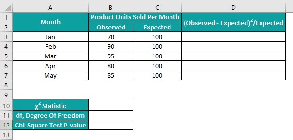
The steps to perform the Goodness of Fit Test are as follows:
Step 1: We need to calculate Chi-Square statistic data points to determine the Chi-Square statistic value in cell B10. So, select cell D3, enter the formula =((B3-C3)^2)/C3, and press Enter.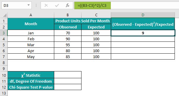
Drag the formula from cell D3 to D7 using the fill handle.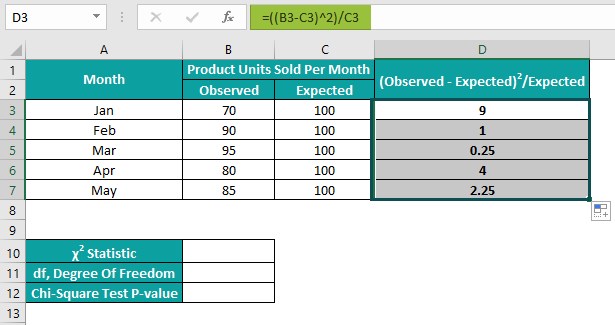
Step 2: Select cell B10, enter the formula =SUM(D3:D7) to add the data points and get the Chi-Square statistic, and press Enter.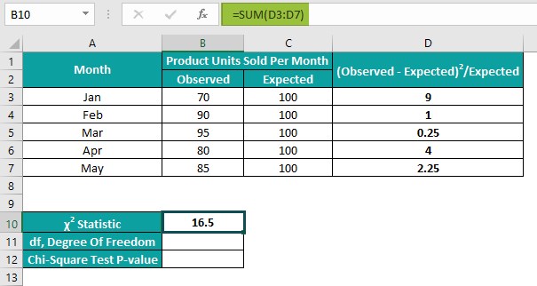
Step 3: Next, as the observations are in 5 rows and 1 column, we can calculate the degree of freedom in the following way. Select cell B11, enter the formula =(5-1), and press Enter.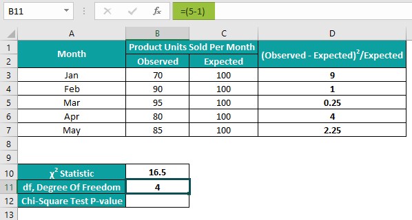
Step 4: Select cell B12, enter the CHISQ.DIST.RT() formula =CHISQ.DIST.RT(B10,B11) to get the Chi-Square Test p-value, and press Enter.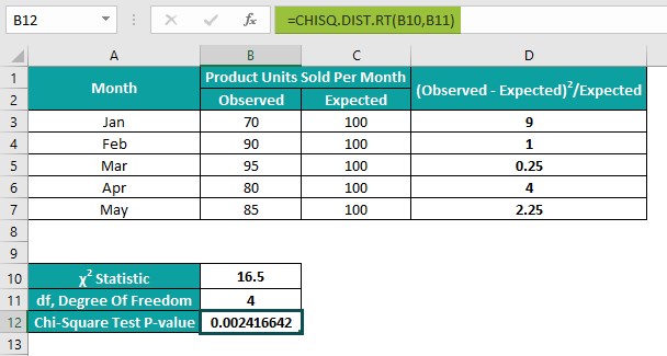
[Output Observation: The CHISQ.DIST.RT() takes the calculated Chi-Square statistic and degree of freedom as the input. It returns the right-tailed probability (p-value) of the Chi-Square distribution for the test statistic 16.5 as 0.002416642. And as the determined p-value is less than the significance threshold of 0.05, we can reject the null hypothesis. It means that the actual number of product units the dealer sells per month differs from the count he claims to sell.]
We can interpret the Chi-Square Test p-value in the following way.
• If the p-value is lesser than or equal to the significance threshold, we can dismiss the null hypothesis and accept the alternative hypothesis.
• If the p-value exceeds the significance threshold. Then, we cannot reject the null hypothesis.
Use this Chi-Square Test In Excel Template to follow along with the examples in this article.
Download Excel Template