What Is SKEW Function In Excel?
The SKEW function in Excel measures the irregularity or asymmetry of the distribution of the data. It evaluates the standard deviation of the logarithms of the individual values of the given dataset. The SKEW Excel function is an inbuilt Statistical function, so we can insert the formula from the “Function Library” or enter it directly in the worksheet.
For example, we will calculate the skewness of the data using the SKEW function.

Select cell B2, enter the formula =SKEW(A2:A5), and press the “Enter” key. The result is “0”, as shown below.
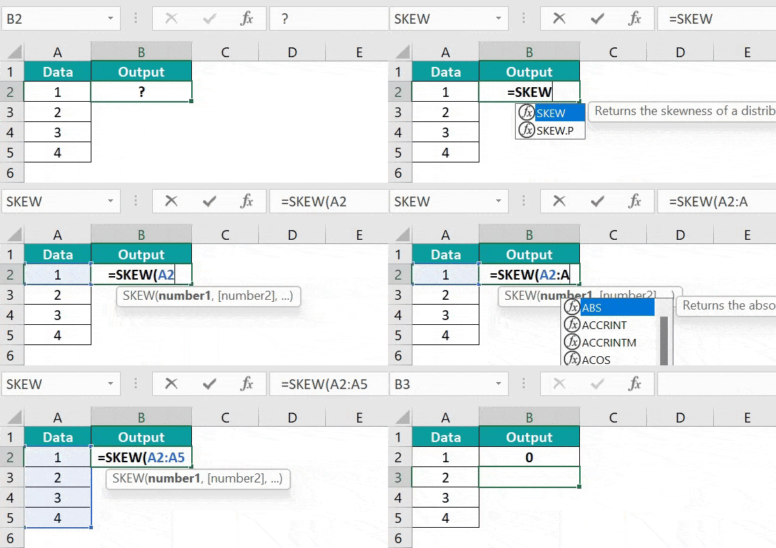
Table of contents
Key Takeaways
- The SKEW Excel function calculates the mean or average of specific values in a dataset.
- An argument that contains error values or text that cannot be translated into numbers returns errors.
- The arguments of the function can be numbers, names, arrays, or cell references that contain numbers.
- We get 3 kinds of SKEW results, namely,
- Perfect SKEW – Equal distribution.
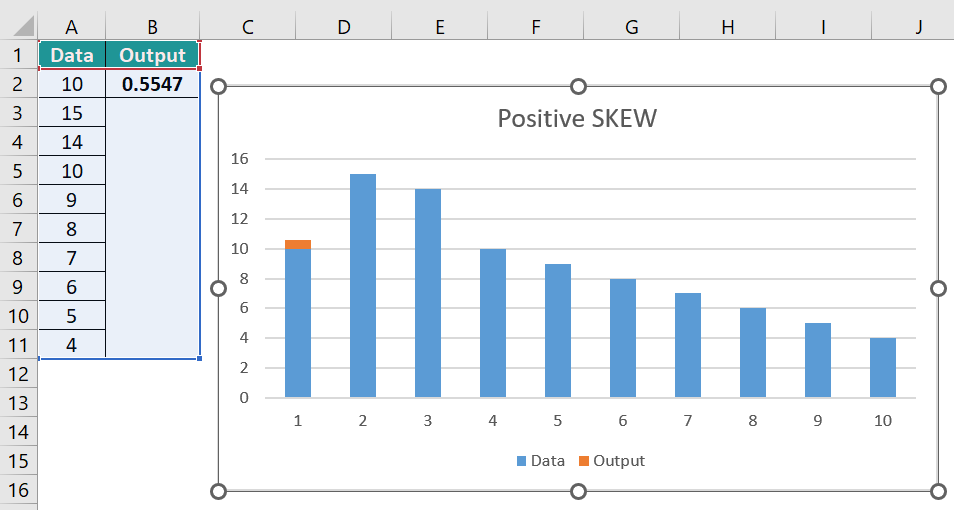
- Positive SKEW – The distribution that is more towards the right.
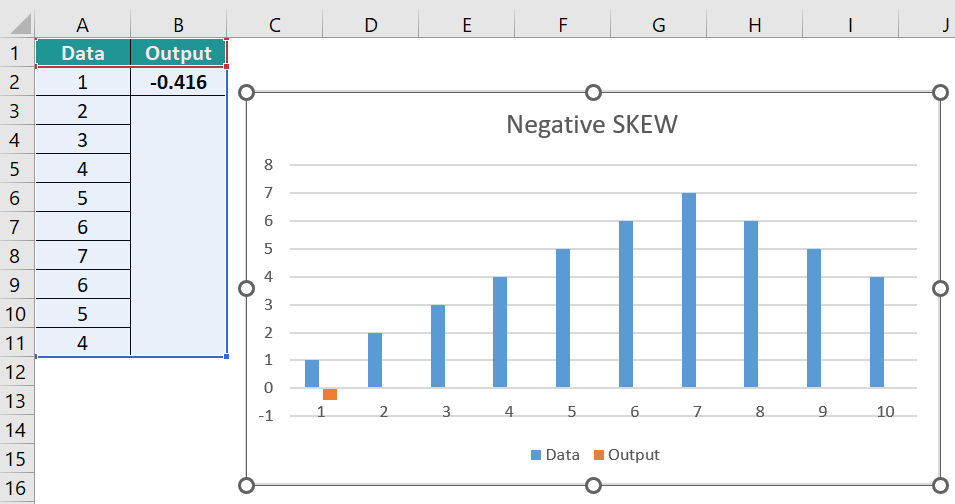
- Negative SKEW – The distribution that is more towards the left.
- The equation for calculating skewness is defined as:

SKEW() Excel Formula
The syntax of the SKEW Excel formula is,

The argument of the SKEW Excel formula is,
- number1, number2,: The first number is the mandatory argument. This argument contains 1 to 255 values that we want to calculate the skewness.
How To Use SKEW Excel Function?
We can use the SKEW Excel function in 2 ways, namely,
- Access from the Excel ribbon.
- Enter in the worksheet manually.
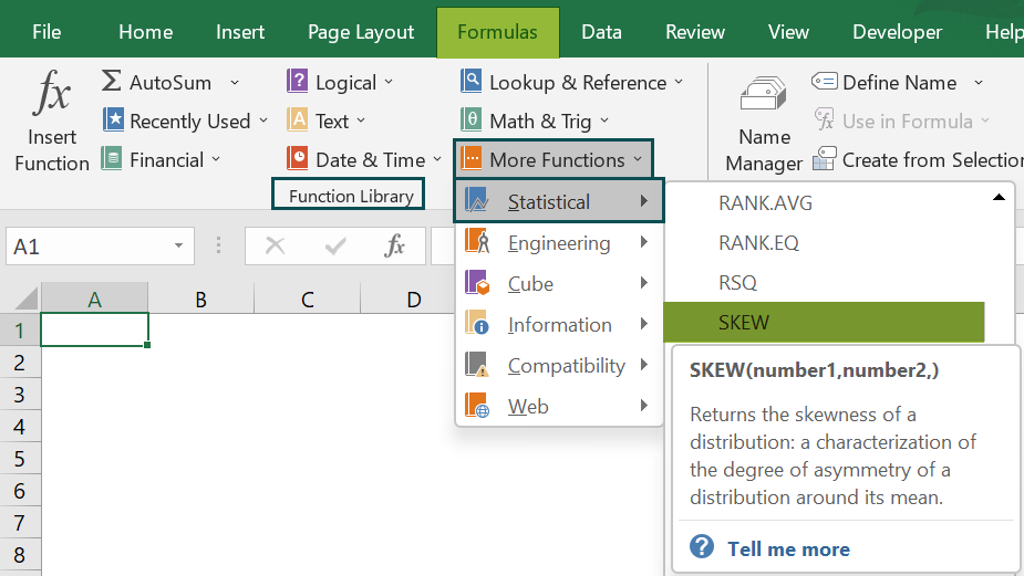
Method #1 – Access from the Excel ribbon
Choose an empty cell for the output → select the “Formulas” tab → go to the “Function Library” group → click the “More Functions” option drop-down → click the “Statistical” option right arrow → select the “SKEW” function, as shown below.
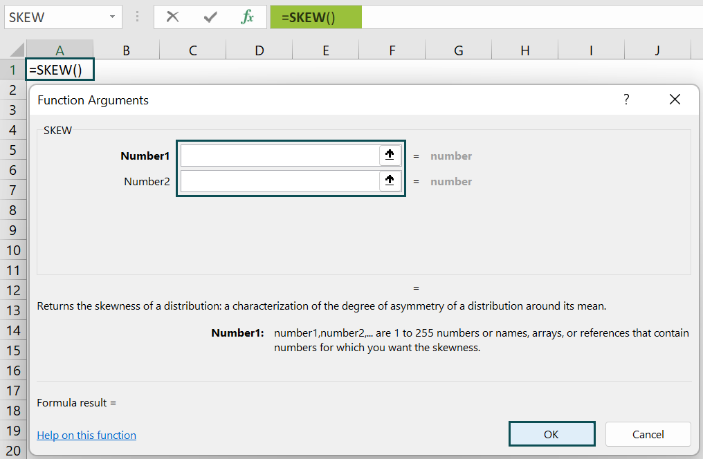
The “Function Arguments” window appears. Enter the arguments in the “number1, number2” fields → click “OK”, as shown below.
Method #2 – Enter in the worksheet manually
- Select an empty cell for the output.
- Type =SKEW( in the selected cell. [Alternatively, type =S and double-click the SKEW function from the list of suggestions shown by Excel.]
- Enter the arguments as cell values or cell reference and close the brackets.
- Press the “Enter” key.
We will calculate the value in the correct format using SKEW Excel function for the student scores.
In the table, the data is,
- Column A contains the Name.
- Column B contains the Score.
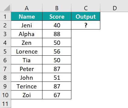
The procedure to calculate the value using SKEW formula is,
- Select cell C2, enter the formula =SKEW(B2:B10), i.e., the number value, and press the “Enter” key.

The result is “0.3876”, as shown above.
Examples
We will understand some advanced scenarios using the SKEW Excel function examples.
Example #1
We will calculate and compare them with the graphical representation using the SKEW function for the two datasets.
In the table, the data is,
- Column A contains Data A.
- Column B contains Data B.

The procedure to calculate the value using the SKEW formula is,
Step 1: First, select cell A6, enter the formula =SKEW(A2:A5), and press the “Enter” key.

Step 2: Next, drag the formula horizontally from cell A6 to B6 using the Excel fill handle.
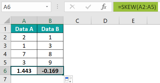
The results in cell A6 as “1.443” and in cell B6 as “0.169”, as shown in the above images.
The graphical representation of the results is shown in the below image.

Example #2
We will calculate the value in the correct format using the SKEW function for the positive output data.
In the table, the data is,
- Column A contains the Data.
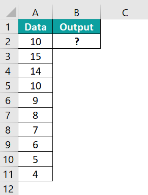
The procedure to calculate the value using the SKEW formula is,
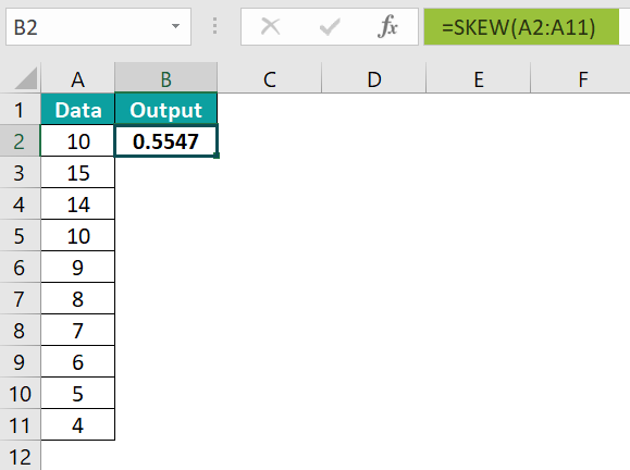
Step 1: Select cell B2, enter the formula =SKEW(A2:A11), and press the “Enter” key. The result is “0.5547, as shown above.
The positive SKEW graphical representation is shown below.
Example #3
We will calculate the value in the correct format using the SKEW function for the negative output data.
In the table, the data is,
- Column A contains the Data.
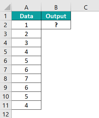
The procedure to calculate the value using the SKEW formula is,
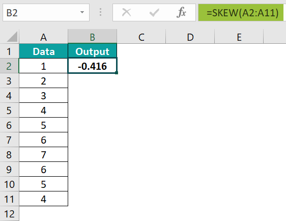
Step 1: Select cell B2, enter the formula =SKEW(A2:A11), and press the “Enter” key. The result is “-0.416”, as shown below.
The negative SKEW graphical representation is shown below.
Example #4
We will calculate the value in the correct format using the SKEW function for the data.
In the table, the data is,
- Column A contains the Data.

The procedure to calculate the value using the SKEW formula is,
Step 1: Select cell B2, enter the formula =SKEW(A2:A11), and press the “Enter” key. The result is “-0.464”, as shown below.

The SKEW graphical representation is shown in the below image.

Important Things To Note
- The “#DIV/0!” error occurs when there are less than three data points or the sample standard deviation is zero.
- An array or reference cell argument containing text, logical, or empty cell values is ignored for calculation, however, the cells containing the value 0 are included for calculation.
- We get “NAME?” and #VALUE! errors when the arguments are entered as cell values, and any one of the values is non-numeric or is not recognized as a number.

Frequently Asked Questions (FAQs)
The SKEW Excel function is used to calculate the standard deviation of the given data.
The syntax of the SKEW function is =SKEW(number1,[number2],…)
The SKEW function can be used as follows:
1) Select an empty cell for the output.
2) Type =SKEW( in the selected cell. [Alternatively, type =S and double-click the SKEW function from the list of suggestions shown by Excel.]
3) Enter the arguments as cell values or cell references and close the brackets.
4) Press the “Enter” key.
For example, we will calculate the value in the correct format using the SKEW function.
In the table, the data is,
• Column A contains the Data.
The procedure to calculate the value using the SKEW formula is,
Select cell B2, enter the formula =SKEW(A2:A4), and press the “Enter” key.
The result is “0.8277”, as shown above.
We can find the SKEW Excel function as follows:
Choose an empty cell for the output → select the “Formulas” tab → go to the “Function Library” group → click the “More Functions” option drop-down → click the “Statistical” option right arrow → select the “SKEW” function, as shown below.
Download Template
This article must help understand the SKEW Excel function’s formula and examples. You can download the template here to use it instantly.
Recommended Articles
This has been a guide to SKEW Excel Function. Here we explain how to use SKEW formula along with examples & downloadable excel template. You can learn more from the following articles –


Leave a Reply