
What is CHOOSEROWS in Google Sheets?
CHOOSEROWS in Google Sheets is a function that allows users to extract specific rows from a given range or array based on their index numbers. This function is particularly useful for dynamically selecting and displaying a subset of data without manually copying, pasting, or filtering. The primary purpose of CHOOSEROWS is to streamline data management and analysis by enabling the quick extraction of relevant rows for reports, dashboards, or focused analysis, without altering the original dataset.
Input this formula in B7: =CHOOSEROWS(A1:B5, 1, 2, 4). You get the selected rows, 1, 2, and 4 in the range.

Use this CHOOSEROWS in Google Sheets Template to follow along with the examples in this article.
Download Excel TemplateSyntax
The function is straight forward. The CHOOSEROWS in Google Sheets formula is as follows:
=CHOOSEROWS(array, row_num1, [row_num2, …])
- array: This is the range or array from which we must extract rows.
- row_num1, [row_num2, …]: These are the index numbers of the rows you want to select from the array. The counting of rows begins from 1 which is the first row of the specified array. One can specify multiple row numbers, even non-contiguous ones, and repeat row numbers to display the same row multiple times.
How to Use CHOOSEROWS Function in Google Sheets?
The CHOOSEROWS function is to return specific rows from a range based on their position. It is used for scenarios where we must select the first few rows of a dataset, extract every nth row, or pick only certain rows without manually copying them.
To enter the CHOOSEROWS in Google Sheets, there are two main ways:
- Enter CHOOSEROWS manually
- From the Google Sheets menu
Enter CHOOSEROWS Manually
To use CHOOSEROWS in Google Sheets manually, we will explain with a simple example. Follow these steps:
Step 1: Create a table with column headers, as shown below. For example, we list items with the fields Item, Quantity, and Price.

Step 2: Click on the cell where you want the result to appear. Type =CHOOSEROWS( as shown below.
=CHOOSEROWS(

Step 3: Now enter the array (your data range) and the row numbers you want to return. You can specify a single row number or multiple row numbers.
=CHOOSEROWS(A2:C7, 1, 3, 5)

Step 4: Press Enter. The function will return rows 1, 3, and 5 from the selected range. Since, we have not selected the header in the range, the first row is the first row of the range, A2:C7.

Entering CHOOSEROWS Through the Menu Bar
- Go to the Insert tab. Choose Function -> Lookup.
- From the list, select CHOOSEROWS.
- A tooltip will appear asking for two arguments: array and row numbers.
- Fill them in with the proper cell ranges and row positions.
- Press Enter to get the result.
Thus, you can extract specific rows from your dataset easily instead of manually selecting them.
Examples
The primary purpose of CHOOSEROWS in Google Sheets is to allow users to select and return specific rows from a specified range. Imagine a scenario where there is a massive dataset. If you wish to have only the fifth, tenth, and fifteenth(or any such high number) rows, instead of manually copying and pasting, we can use CHOOSEROWS to do it with ease.
Example #1
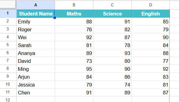
The CHOOSEROWS function pulls out only the required rows from a larger dataset. For instance, if you have a list of students and their grades in 3 subjects. Here, we wish to display the fifth and tenth rows, and the fifth row again. We use CHOOSEROWS to make this simple without manually copying data.
Step 1: Set up your database using the headers Name, Maths, Science, and English. Enter some sample data as shown below:
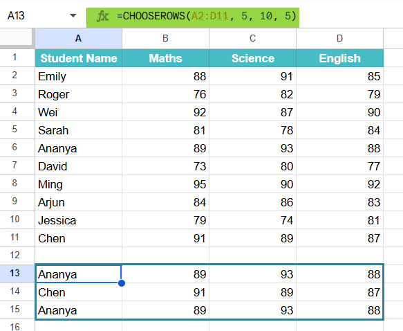
Step 2: Click on an empty cell from which we will get the results of the selected rows. Type the following formula:
=CHOOSEROWS(A2:D11, 5, 10, 15)
A2:D11 is the range.
5,10,5 are the row positions within that range you want to extract.

Step 3: Press Enter. The function will return rows 1, 3, and 5 from the dataset:
Example #2 – Using CHOOSEROWS to Extract the First and Last Rows
One of the unique features of CHOOSEROWS is its ability to return rows from both the beginning and the end of a dataset. When we use large spreadsheets, we can find the first and last entries instantly with a simple formula instead of scrolling through them. This is especially useful when you want to check the earliest and most recent records in your data.
Step 1: Set up the table as shown below. We have some items their quantity and price.

Step 2: Click on the cell where you want the result to appear. Type the following formula:
=CHOOSEROWS(A2:C9, 1, -1)

Here, the first argument A2:C9 is the range.
- 1 extracts the first row.
- -1 extracts the last row. Here, negative numbers count from the bottom of the range.

Step 3: Press Enter. The function will return the first and last rows from the dataset:
With CHOOSEROWS, you can pull out both the first and last entries in a dataset. This unique feature saves time when tracking opening and closing balances, earliest and latest dates, or beginning and end records in large spreadsheets.
Example #3 – Using CHOOSEROWS with ARRAYFORMULA Function
While CHOOSEROWS works well for extracting rows by position, sometimes you may want to first filter the data and then apply CHOOSEROWS to pick specific rows from that filtered output. By combining FILTER with ARRAYFORMULA and CHOOSEROWS, one can achieve this easily without manually adjusting ranges.
Step 1: Enter all the required details as shown below. In this example, we enter the details of a shop’s products and their corresponding prices.

Step 2: We only want rows where the price is greater than $2. And from this, we must first extract the first and third rows from that filtered list. Enter the following formula:
=CHOOSEROWS(FILTER(A2:C7, B2:B7>2), 1, 3)

Step 3: Press Enter. The FILTER function creates a new dataset where Price > 2, and then CHOOSEROWS picks rows 1 and 3 from that filtered list.

Step 4: You can also wrap the entire formula in ARRAYFORMULA in case you want to dynamically expand and adjust when more rows are added:
=ARRAYFORMULA(CHOOSEROWS(FILTER(A2:B100, B2:B100>12), 1, -1))
This ensures the formula keeps working even when more products are added to your dataset. Below, we have added the last entry “Pastry” dynamically. It has however been chosen as the last row to display due to the addition of ARRAYFORMULA.

By combining FILTER, ARRAYFORMULA, and CHOOSEROWS, one can extract non-contiguous rows dynamically from filtered data. This is a powerful way to automate reports and display only the rows that matter.
Important Things to Note
- If you specify a row number that exceeds the available range, Google Sheets will throw an error. For this, you can use ARRAYFORMULA and give a bigger range.
- CHOOSEROWS works best with contiguous ranges. If you need non-contiguous rows, consider using FILTER to achieve the same result.
- CHOOSECOLS function creates a new array from the selected columns in the existing range.
- One can use cell references instead of hardcoding row numbers. For instance, if cell D1 contains the row number you want, use =CHOOSEROWS(A2:F6, D1).
- Sometimes one may get errors if the row numbers exceed the given range. Use IFERROR to handle them.
- If you frequently use the same range, define it as a named range. This makes your formulas cleaner and easier to read.
Frequently Asked Questions (FAQs)
1. The function can be used to analyze survey responses and to extract specific rows for respondents giving positive feedback like “Yes.” We can combine FILTER with CHOOSEROWS for this, as seen in Example 3.
2. Organizations can use CHOOSEROWS to pull only the most recent entries from a large sales log,
3. HR teas or schools can use it to highlight selected rows, like top-performing students or employees with the highest ratings.
Yes. For this, we can use negative numbers.
=CHOOSEROWS(A2:B10,
-1) This returns the last row of the range.
We use CHOOSEROWS to pick rows by position (e.g., row 1, 3, 5). Here, you must know exactly which rows you want.
We use the FILTER function to pick rows based on conditions (e.g., Quantity > 10). Here, you do not have to know the row number, but only the condition.
Use this CHOOSEROWS in Google Sheets Template to follow along with the examples in this article.
Download Excel Template