
What Is Drop Down List In Excel?
Drop-down list in Excel is used to ease users’ work by giving options to select an item instead of typing the values everytime.
Excel spreadsheets are often used as a data entry tool, and collecting data from multiple sources may lead to data discrepancies. If the data received from the sources have discrepancies, it takes a whole lot of time to clean it up. Hence, the concept of data validation through drop down is very much handy.
Download FREE Drop Down List in Excel Template and Follow Along!Use this Drop Down List in Excel Template to follow along with the examples in this article.
Download Excel Template
For example, assume that we have to collect data from employees on a few questions like the following table.

Users should write either YES or NO. But some users entered YES, and some users entered Y, S. There is a data inconsistency here. This is where the drop-down list allows the user to select either YES or NO. We cannot enter anything else.

Drop down list are the pre-defined values created by the admin user. It allows the other user to enter the values that are exactly the same as in the drop-down list. By using drop-down lists, admin users can get error-proof data inputs from other users.
Key Takeaways
- The drop-down list helps users select an item from the options instead of typing the values.
- It can be created using cell reference as well as by entering the values directly into the source box.
- Drop down list will not allow the user to enter the values apart from the values available in the list.
- The list makes the entries error-proof. To make the user aware of the validation rule, we can display an input message box and include an error message.
- Users either select the values from the drop-down or enter the values that are there in the drop-down list manually.
How To Create Drop Down List In Excel?
Let us explain the process of creating a simple dropdown list in Excel.
Example #1 – Create Drop Down List Without Cell Reference
For example, assume we need to create a drop-down list of YES or NO for the user to choose. Assume, the following questions are the data.

Users should be allowed to select or enter only YES or NO. Follow the steps listed here:
Step 1: Select the cells from B2:D3.

Step 2: Go to the Data tab, and under the data tools, click on Data Validation.

Step 3: The Data Validation excel window opens up. Choose List from the Allow: dropdown list.

Step 4: In the Source: box, enter the dropdown values i.e., YES and NO, each separated by a comma (,).

Step 5: Click on OK, and the dropdown list will appear for all the selected cells.

Now, we cannot enter any other value apart from YES or NO.
If they try to enter any values apart from the ones available in the drop-down, Excel will show the following warning message.

The warning message says, ‘This value doesn’t match the data validation restrictions defined for this cell’.
This is the default message user will get. However, we can modify this and give our own warning message.
Modify The Warning Message
Step 1: Again, select all the dropdown applied cells i.e., B2:D3.

Step 2: To bring the data validation window, press the shortcut keys ALT + A + V + V.

Step 3: Click on the Error Alert tab.

Step 4: In the Style drop-down, we can choose the kind of error icons.

We have 3 options under style i.e., Stop, Warning, and Information.
- Stop Error Message Icon
- Warning Error Icon
- Information Error Icon
Step 5: In the Title box, enter the title as Data Validation in Place.

Step 6: In the Error Message: box, write the message that we want to show to the users.

Click on OK. The error message will appear when the user tries to enter the values outside of the drop-down list.

However, we can also design the information message about the data validation applied to the cell as soon as the users select the data validation cell.
In the data validation window, click on the Input Message tab and enter the message we want to display.

Click on OK. It will show the input message whenever users select the data validation cell.

In this way, we can alert the users about the validation rules applied to the specific cell or cells.
Example #2 – Create Drop Down List With Cell References
In the above example #1, we have seen drop-down values directly entered into the source box. However, it will be very difficult to make changes in the cells with data validation, especially if we want to create many values that change regularly.
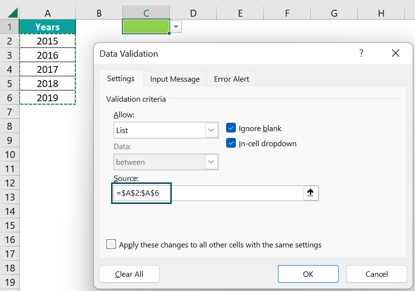
For example, we have the list of city names in Excel.

Let us create a drop-down list by using cell references in excel.
Step 1: Select the desired cell where we want to create the drop-down list. Press the data validation shortcut keys ALT + A + V + V to bring the following data validation window.

Step 2: Choose List from the criteria option and choose the source from A2:A6.

Step 3: Click on OK, and the drop-down list will be ready in cell C1.

The cities available in the range A2:A6 are also available in the drop-down list as well. The advantage of using cell reference as the input source for creating a drop-down list is that whenever changes happen in the source range (A2:A6) automatically impacts the drop-down list as well.
For instance, take a look at the following image.

In cell A4 we have changed the value from London to Durban, and that change is immediately visible in the dropdown list as well.
Edit Drop Down List In Excel
We can edit drop-down lists in excel with ease. For instance, in the following image, we have created the drop-down list based on cells.

As of now, the current cell reference is from A2:A6.
If we want to expand or change the reference of cells, we can click inside the source box and choose the reference that we want.

Previously it was taking the reference of A2:A6; now, we have edited it to A2:A10. So, anything entered in A2:A10 will be reflected in the drop-down list.
Remove Drop Down List In Excel
Creating a drop-down list in Excel ensures some sort of data quality when we need to collect data from multiple users. However, removing them is also a part of the process, because copy-pasting the drop-down cell from one cell to another will create a frustrating experience for the users.
Because when we copy the drop-down cell to another cell, we aren’t copying just the cell; in fact, we are copying the drop-down list as well, along with the rules applied while creating the drop-down cell.
There are several ways we can remove the drop-down in Excel. We will show you one by one starting with a simple technique.
Method 1: Remove Drop Down from Specific Cell
For example, look at the following image that shows the drop-down list in Excel.


After selecting the desired cell, go to the Data tab and click on the Data Validation option.


Click on the Clear All option.

This will clear the drop-down from all the selected cells.
Note: In case the selected cells have multiple drop-downs, then it has removed only the selected drop-down list. The rest of the drop-down lists would remain the same, and we need to do the same steps to remove all of the drop-down lists.
Remove Drop Down Like a Pro Using the Shortcut
We can use the drop-down list by pressing the excel shortcut keys ALT + A + V + V (press one key at a time and do not hold the ALT key).
This will bring the Data Validation window, then click on the “Clear All” button to remove the drop-down.
Method 2: Use Clear All Button
In the previous example, we removed just the data validation from the selected cell, however, there is a clear all button available to remove all drop downs along with values and formatting from the selected cell or cells.
Select the cell or cells that we would like to remove from the drop-down list.
In the image above, in cell C1 we have a drop down and the value selected from the drop-down is “May”.
After the cell or cells are selected, go to the Home tab, and under the Editing section, we have a clear icon.

Click on the Clear button to see the options in this icon.

We have several options and click on Clear All to see the effect of it in cell C1
Everything in cell C1 will be removed as soon as we click the Clear All button. Right from the drop-down list, the value we had in cell C1, and also the formatting applied to cell C1.
If we need to start something afresh in the worksheet, we can use this method. Otherwise, we may lose out on data.
The shortcut key to apply the Clear All feature is ALT + H + E + A (press one key at a time and do not hold the ALT key).
Method 3: Use Copy and Paste Method
We can use the copy-and-paste method to remove the drop-down list from the cell. When we copy one cell to another, we usually copy everything from that cell and paste it to the destination cell.
For example, in the following image, we have a drop-down in cell C1.
To remove the drop-down from this cell, copy any of the blanks in the worksheet. For example, say we copied cell C2.
After cell C2 (blank cell) was copied, select the target from which we would like to have a drop-down i.e., cell C1.
Right-click on the targeted cell and click on the paste option.
In the drop-down list from cell C1, all the formatting and values will be removed.
Likewise, by using various methods, we can remove the drop-down list in Excel.
Create Dynamic Drop Down List In Excel?
With normal cell reference, the drop-down list is not dynamic. Whenever new entries are added to the current drop-down list, it does not show the newly added items.
For instance, the following image shows the dropdown list references cell ranges from A2:A5.

If we add a couple of entries in cells A6 and A7, the current reference will not reflect in the dropdown list.

We have added new country names in cells A6 and A7, but the drop-down list is not showing them. When the dropdown list is created, it is referenced from A2:A5. Anything added after cell A5 will not be visible in the drop-down list.
To fix this, we need to create a dynamic dropdown list in excel by using the OFFSET function.
Step 1: Open the data validation window by pressing the shortcut keys ALT + A + V + V.

Step 2: In the source box, enter the following formula.
=OFFSET($A$2,0,0,COUNTA($A$2:$A$1048576))

Step 3: Click on OK, and the dynamic drop-down list is ready.

Now add new entries to the list.

As soon as we have added new entries, the drop-down list is showing the newly added items dynamically.
OFFSET Formula Explanation: The formula we have used is
=OFFSET($A$2,0,0,COUNTA($A$2:$A$1048576))
The OFFSET formula syntax read like this.
OFFSET(Reference, Row, Column, Height, Width)
The OFFSET function in excel starts its reference from cell A2.
It moves zero rows down.
It moves zero columns right.
To determine how many cells are filled up with values, the COUNTA excel function will check the number of filled rows count in the entire column A. Then, it returns the number of filled rows count, and then the OFFSET function will offset those many rows and return a bunch of rows.
In this way, we can create a dynamic dropdown list in Excel.
Important Things to Note
- ALT + A + V + V is the shortcut key to activate the data validation window.
- When we copy the dropdown cell and paste it into other cells, then, the dropdown list in excel will also be copied.
- When we copy the non-drop-down cell and paste it on the drop-down cell, it will be taken away.
- We can copy the dropdown list on excel based on paste special in excel.
- The input message will display the validation rule applied to the cell or cells.
Frequently Asked Questions (FAQs)
Unfortunately, there is no way, we can create a dropdown list in excel without data validation. In fact, the drop-down list is there to check the kind of data the user enters.
Dropdown lists are used in Excel to have data consistency from the users. All the users will be entering the values only from the pre-defined values, and data will be neat and clean for all the users.
The drop-down list can hold up to 32,767 values, and it is highly unlikely any of the users use those many entries.
If you want to select multiple values from the dropdown list, then with default features, we cannot select them. However, by using VBA code, one can make multiple selections from the drop-down list in Excel.
Use this Drop Down List in Excel Template to follow along with the examples in this article.
Download Excel Template