
What Is Freeze Panes In Excel?
The Freeze Panes in Excel is a feature that freezes the row’s or the column’s position so that they remain fixed even when we scroll down or up to see the whole sheet.
The frozen columns and rows remain on the screen in the same place. This feature is helpful while working in a large dataset.
Use this Freeze Panes in Excel Template to follow along with the examples in this article.
Download Excel TemplateFor example, let us consider the below table listing the total marks obtained by students in four semesters in columns A, B, C, D, and E, respectively. We need to use the following steps to freeze the top row (row 1) in excel.

- Step 1: Go to the View tab in excel.
- Step 2: Choose Freeze Panes from the Window group.
- Step 3: Select the Freeze Top Row option from the dropdown list.
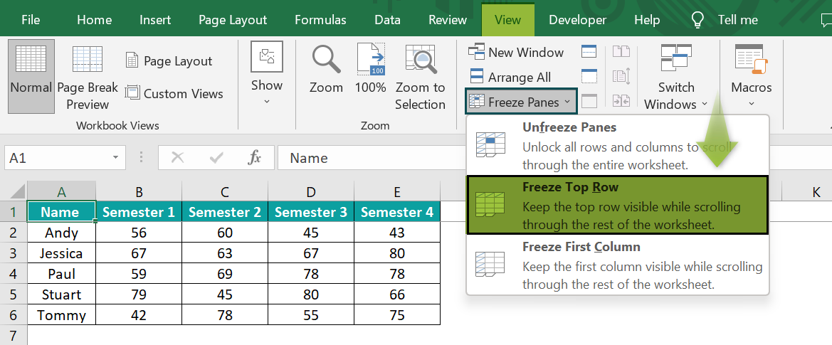
The Freeze Top Row option freezes the top row.
Key Takeaways
- The Freeze Panes in Excel fix the position of the rows and the columns in the table.
- There are three freeze panes options:
- Freeze Panes
- Freeze Top Row
- Freeze First Column
- We should select the adjacent cell to the desired row or column to freeze.
- In the Freeze Panes, we can freeze rows and columns on the same or multiple sheets.
- We can unfreeze the frozen rows or columns using View → Freeze Panes (from the Window group) → Unfreeze Panes.
How To Freeze Rows In Excel?
We can use the following steps to freeze rows in excel;
- Add the data to the excel worksheet.
- Go to the View tab in Excel.
- Choose Freeze Panes from the Window group.
- Select the Freeze Top Row option from the dropdown list.

We can freeze the header row and multiple rows in excel using the freeze panes option.
Let us understand the method to freeze rows in excel with the following examples.
Example #1 – Header Row
The below table shows the personal data of people such as Name, Age, Gender, Qualification, and Monthly Income in columns A, B, C, D, and E, respectively. We need to use the following steps in Excel to understand how we can freeze Header Row in excel.

The steps used to freeze the header row in excel are as follows:
- Step 1: Add the data on the sheet.
- Step 2: Go to the View tab.
- Step 3: Choose Freeze Panes from the Window group.
- Step 4: Select the Freeze Top Row option from the dropdown list.

- Step 5: The Freeze Top Row option freezes the header row’s position to remain fixed. When we scroll down the worksheet, all the successive rows scroll up except the header row.
For instance, consider the below image, where we can see row 3 after row 1. It is because row 3 moves up when we scroll and hides row 2. But row 1 stays visible on the screen at the same position.

- Thus, we can freeze the header row (row 1) using freeze panes in excel.
Example #2 – Multiple Rows
The following table shows the sales recorded by people at different places. We need to use the below steps in excel to freeze multiple rows of excel.
In the table,
- Column A indicates the names of the people
- Column B shows the sales records
- Column C displays the countries

The steps used to freeze multiple rows in excel are as follows:
- Step 1: We should select the row below the one we want to freeze.
In this example, let us freeze the first two rows. So, we need to select row 3.
- Step 2: Go to the View tab.
- Step 3: Choose Freeze Panes from the Window group.
- Step 4: Select the Freeze Panes option from the dropdown list.

- Step 5: The Freeze Panes option freezes the first two rows’ positions such that they remain fixed. When we scroll down the worksheet, all the successive rows scroll up except the first two rows.
For instance, consider the below image, where we can see row 4 after row 2. It is because row 4 moves up when we scroll and hides row 3. But rows 1 and 2 remain visible on the screen at the same position.

- Thus, we can freeze multiple rows using freeze panes in excel.
How To Freeze Columns In Excel?
Similar to rows, we can also freeze columns in excel.
We can use the following steps to freeze columns in excel.
- Add the data to the sheet.
- Go to the View tab in Excel.
- Choose Freeze Panes from the Window group.
- Select the Freeze First Column option from the dropdown list.

We can freeze the first column (A) or multiple columns in excel using the Freeze Panes option, available under the Window group.
Let us understand the method to freeze columns in excel with the following examples.
Example #1 – First Column
The below table shows a person’s bank transactions, such as deposits and withdrawal amounts. We need to use the following steps to freeze first column in excel.
In the table,
- Column A displays the date
- Column B indicates the transactions, titled item
- Column C shows the amount

The steps used to freeze the first column in excel are as follows:
- Step 1: Add the data on the sheet.
- Step 2: Go to the View tab.
- Step 3: Choose Freeze Panes from the Window group.
- Step 4: Select the Freeze First Column option from the dropdown list.

- Step 5: The Freeze First Column option freezes the first column position such that it remains fixed. When we scroll right, all the successive columns scroll to the left, except the first column.
For instance, consider the below image, where we can see column C after column A. It is because column C moves to the left when we scroll and hides column B. But Column A stays visible on the screen at the same position.

- Thus, we can freeze the first column using freeze panes in excel.
Example #2 – Multiple Columns
The following table shows the employee’s details of a company, such as employee’s IDs, Date, Location, Age, and Gender in columns A, B, C, D, and E, respectively. We need to use the following steps in Excel to freeze multiple columns in excel.

The steps used to freeze multiple columns in excel are as follows:
- Step 1: We need to select the column that is present right to the column we want to freeze.
In this example, let us freeze the first two columns. So, we need to select column C.
- Step 2: Go to the View tab.
- Step 3: Choose Freeze Panes from the Window group.
- Step 4: Select the Freeze Panes option from the dropdown list.

- Step 5: The Freeze Panes option freezes the first two columns’ positions such that they remain fixed. When we scroll left, all the successive columns scroll except the first two columns.
For instance, consider the below image, where we can see column D after column B. It is because column C moves left when we scroll. But columns A and B remain visible on the screen.

- Thus, we can freeze multiple columns using freeze panes in excel.
How To Freeze Rows And Columns?
Let us understand how to freeze panes both column and row on the same datasheet.
For example, the below table shows the price of various fruit. Column A indicates the names of fruits, and columns B, C, and D show the price/unit, unit, and total cost values. We need to use the following steps in Excel to freeze rows and columns in excel.

The steps used to freeze rows and columns in excel are as follows:
- Step 1: Add the data on the sheet.
- Step 2: We need to select the cell adjacent to the rows and columns we want to freeze.
In this example, let us freeze row 1 and column A. So, we need to select cell B2.
- Step 3: Go to the View tab.
- Step 4: Choose Freeze Panes from the Window group.
- Step 5: Select the Freeze Panes option from the dropdown list.

- Step 6: The Freeze Panes option freezes the selected row’s and column’s positions to remain fixed.
When we scroll up and down, all the successive rows scroll up except row 1.
For instance, consider the below image, where we can see row 3 after row 1. It is because row 3 moves up when we scroll and hides row 2. But row 1 stays visible on the screen at the same position as shown below.

- Step 7: Similarly, when we scroll left to right, all the successive columns scroll up except column A.
For instance, consider the below image, where we can see column C after column A. It is because column C moves left when we scroll and hides column B. But column A stays visible on the screen at the same position.

- Therefore, we can freeze the rows and columns on the same datasheet using the freeze panes option.
Unfreeze Panes In Excel
Let us consider an example to understand how to unfreeze panes in excel.
The below table shows the list of items (in column A) along with their prices (in column B). We need to use the following steps in Excel to unfreeze panes in excel.

To understand the steps to unfreeze panes in excel, let us first freeze the rows and the columns.
The steps used to freeze rows and columns in excel are as follows:
- Step 1: Add the data on the sheet.
- Step 2: We need to select the cell adjacent to the rows and columns we want to freeze. In this example, let us freeze column A along with rows 1 and 2. So, we need to select cell B3.
- Step 3: Go to the View tab.
- Step 4: Choose Freeze Panes from the Window group.
- Step 5: Select the Freeze Panes option from the dropdown list.

- Step 6: The Freeze Panes option freezes the selected row’s and column’s positions to remain fixed.
When we scroll up and down, all the successive rows scroll up except rows 1 and 2. It is because row 4 moves up when we scroll and hides row 3. But row 2 remains visible on the screen at the same position.

- Step 7: Similarly, when we scroll left to right, all the successive columns scroll up except column A.
For instance, consider the below image, where we can see column C after column A. It is because column C moves when we scroll and column B. But column A stays visible on the screen at the same position.
As we can see, the data have only two columns (A and B); since column B is hidden, the only visible column is column A.

As we have frozen the rows and columns, we can now learn how to unfreeze the panes in excel.
The steps used to unfreeze panes in excel are as follows:
- Step 1: Go to the View tab.
- Step 2: Choose Freeze Panes from the Window group.
- Step 3: Select the Unfreeze Panes option from the dropdown list.
The Unfreeze Panes option unfreezes the frozen rows and columns.

Important Things To Note
- The Freeze Panes option saves time as users need not repeatedly scroll to see the headers or any important information.
- By freezing the headers of rows and columns, understanding the content of the data is made easier.
- Using this feature, we can easily compare rows and columns of a large dataset.
- We can also use the shortcut to freeze panes in excel.
Frequently Asked Questions (FAQs)
When working in huge datasets, we find it difficult to scroll all the way up to see the column heading or any specific data. The freeze panes option freezes the position of the rows and columns, making it easy to compare as the frozen rows and columns remain visible at all times.
For example, let us consider the below table listing the sales of various products in 4 quarters. Column A indicates the products and columns B, C, D, and E, displays the sales in 4 quarters. We need to use the following steps to freeze the header row in excel.
• Step 1: Add the data to the excel worksheet.
• Step 2: Go to the View tab in excel.
• Step 3: Choose Freeze Panes from the Window group.
• Step 4: Select the Freeze Top Row option from the dropdown list.
• Step 5: The Freeze Top Row option freezes the header row’s position to remain fixed. When we scroll down the worksheet, all the successive rows scroll up except the header row.
For instance, consider the below image, where we can see row 3 after row 1. It is because row 3 moves up when we scroll and hides row 2. But row 1 stays visible on the screen at the same position.
• Thus, we can freeze the header row using freeze panes in excel.
The steps to access the Freeze Panes option in Excel under the Home tab are listed as follows:
a) Go to the View tab of Excel.
b) Choose the Freeze Panes from the Window group
c) Select the Freeze Panes option from the dropdown list.
The shortcut to Freeze Panes in Excel are listed as follows:
• Freeze Top Row – Press the keys ALT + W + F + R to freeze the top row of the table.
• Freeze First Column – Press the keys ALT + W + F + C to freeze the first column of the table.
• Freeze Panes, i.e., both Rows and Columns – Press the keys ALT + W + F + F to freeze both the rows and the columns of the table.
Use this Freeze Panes in Excel Template to follow along with the examples in this article.
Download Excel Template