
What Is F-TEST In Excel?
The F-TEST in Excel determines the two-tailed probability of the variances of the specified array1 and array2 not being significantly different. Users can use the FTEST Excel function to test if two independent datasets belong to a normal population with the same variability.
But the FTEST() got replaced by a more accurate function, F.TEST(), in Excel 2010. So now, the FTEST() is available as a Compatibility function, offering backward compatibility.
Use this FTEST Excel Template to follow along with the examples in this article.
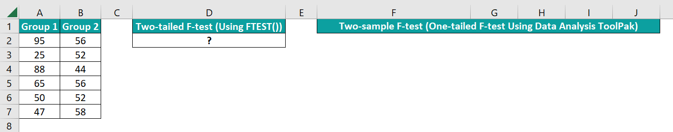
Download Excel TemplateFor example, the first table contains two datasets, Group 1 and Group 2.
Suppose the requirement is to conduct F-Test for the two given datasets. Then, applying the FTEST Excel function in the target cell D2 will give us the two-tailed probability of the two data sets’ variances not being considerably different.
And using the F-TEST Excel feature from the Data Analysis option in the Data tab will give us the one-tailed F-Test result. It will help us decide whether to accept or reject the null hypothesis that the variances of the two datasets are the same.
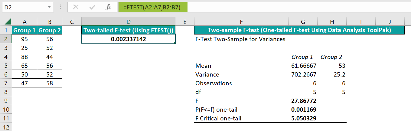
In the above F-Test Excel example, the FTEST function in cell D2 accepts Groups 1 and 2 as the two input arrays. It thus returns the p-value, 0.002337142. It shows the probability of the variances of Group 1 and Group 2 not being significantly different is 0.002337142, or 0.2%. Thus, the value implies that the probability of the variances being significantly different is higher.
On the other hand, the one-tailed F-Test result shows that the p-value is 0.001169, which is less than the significance threshold value (Alpha), 0.05. And the F-value, 27.86772, is greater than the F Critical value, 5.050329.
The above F-Test Excel interpretation is that we must reject the null hypothesis and accept the alternate hypothesis. And the alternate hypothesis could be, say, Group 1 variance is higher than Group 2’s variance, as it is a one-tailed test.
The p-value the FTEST Excel function returns will be double the p-value we get when using the FTEST feature from Data Analysis ToolPak. The reason is that the former is a two-tailed F-Test Excel case, while the latter performs a one-tailed F-Test.
Key Takeaways
- The FTEST Excel function computes the two-tailed probability of the two given arrays’ variances not being considerably different. Users can use the FTEST function to confirm if the two specified datasets have similar or different variances.
- As inputs, the FTEST Excel function accepts two mandatory arguments, array1, and array2.
- The FTEST function is a Compatibility function. It got replaced by a more accurate function, F.TEST(), in Excel 2010.
- The FTEST Excel function performs a two-tailed F-Test. But if you must conduct a one-tailed F-Test to conclude whether to accept or reject the null hypothesis, use the F-Test option in Data → Data Analysis.
FTEST() Excel Formula
The FTEST Excel formula to get the required two-tailed probability value is:
where,
- array1: The first dataset or array of values.
- array2: The second dataset or array of values.
Both the arguments in the FTEST Excel function are mandatory.
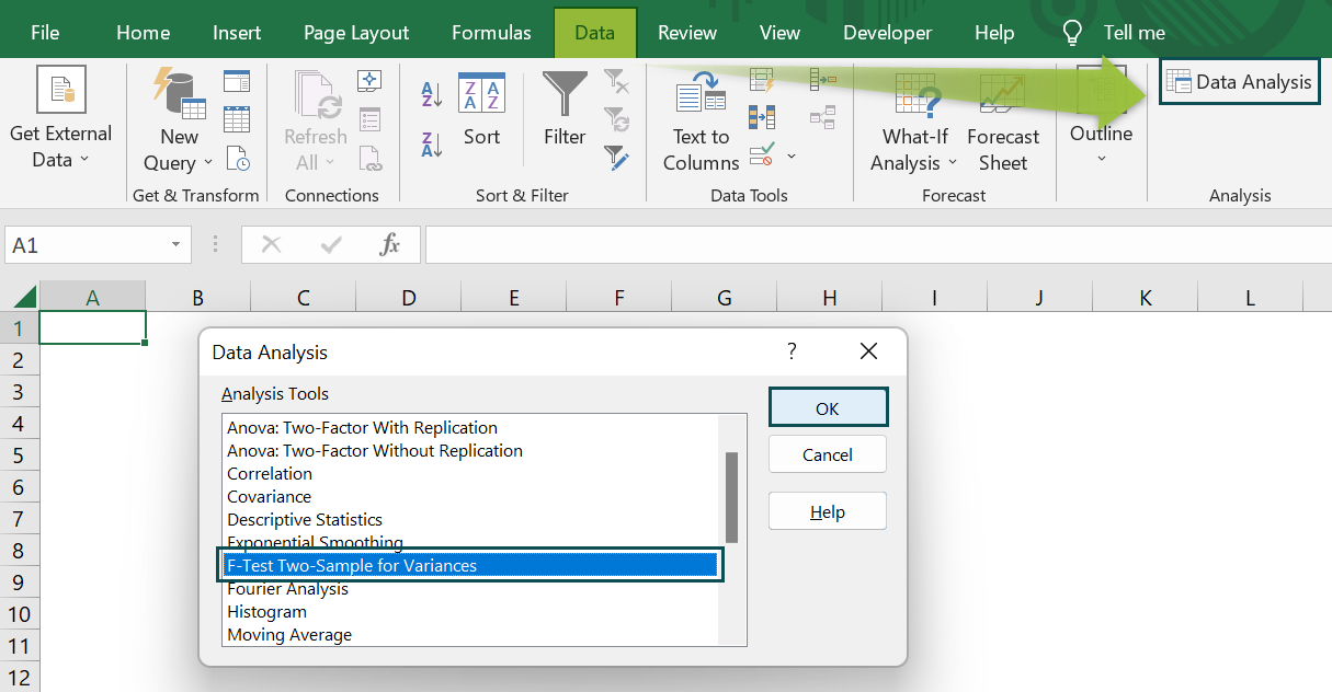
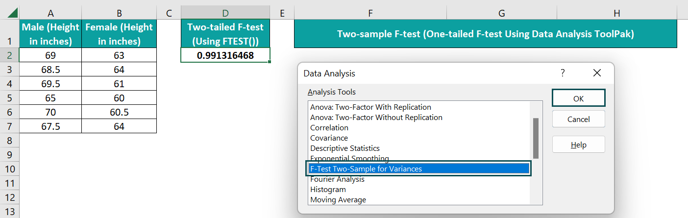
But we must open the Data Analysis window to apply the FTEST function using the Data Analysis feature for performing a one-tail F-Test. And then, select F-Test Two-Sample for Variances option.
This step will open the F-Test Two-Sample for Variances window.
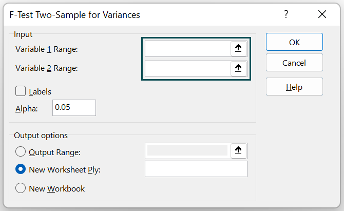
The two variable ranges in the Input section take the two arrays as the input to conduct the F-Test.
How To Do F-TEST in Excel?
The steps to apply the FTEST Excel function are as follows:
- First, ensure the two given arrays contains valid data and have non-zero variances.
- Next, choose the target cell, and enter the FTEST Excel function.
- Finally, press Enter to get the required probability value.
The following F-Test Excel example explains the above steps in detail.
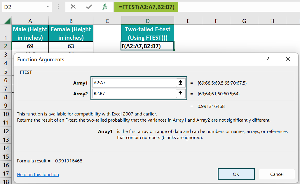
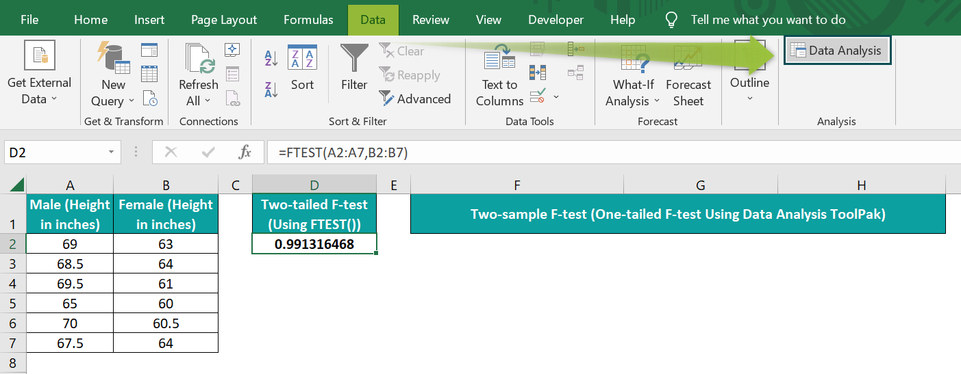
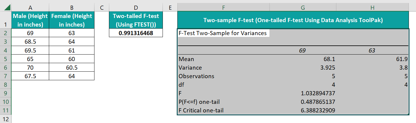
The first table shows male and female sample height values.
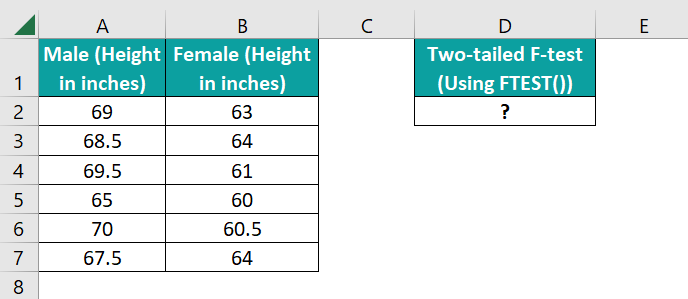
The requirement is to determine the two-tailed probability of the two data sets’ variances not being considerably different and display the output in cell D2. Then, applying the FTEST Excel function in the target cell will get us the required data.
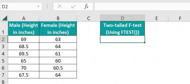
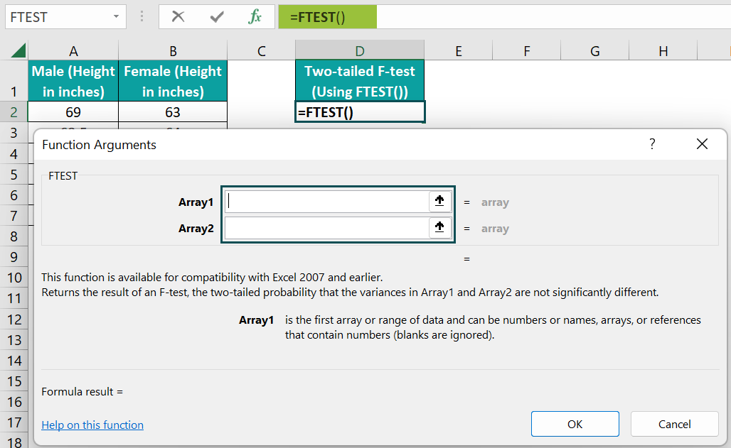
- Step 1: Select the target cell D2, enter the FTEST(), and press Enter.
=FTEST(A2:A7,B2:B7)
The FTEST() returns the probability of the supplied arrays not having significantly different variances as 0.991316468. Thus, the probability of the two datasets having more or less similar variance values is high.
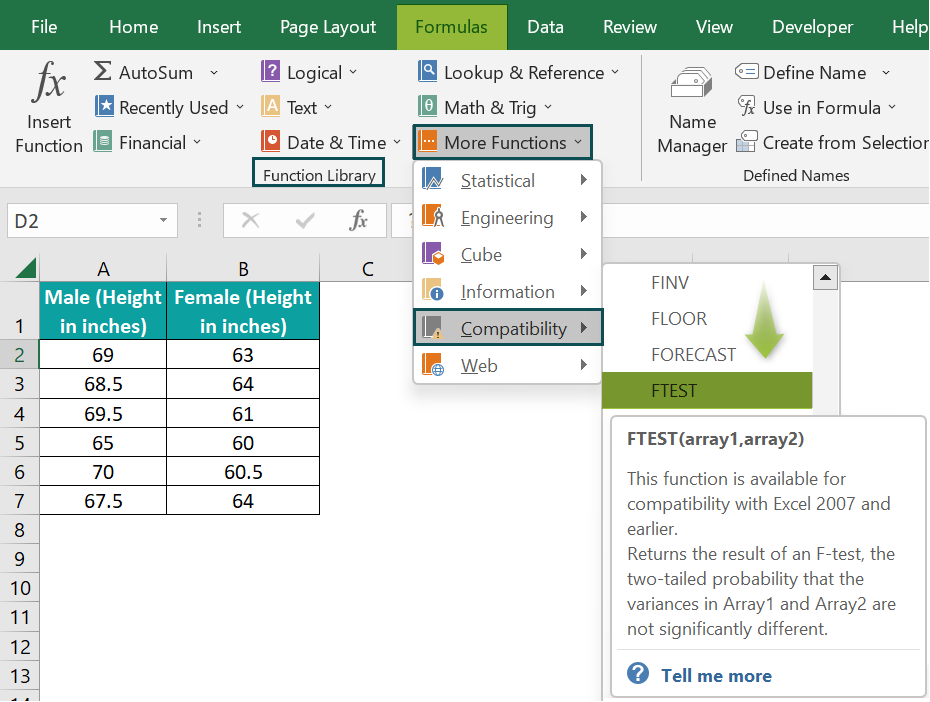
Alternatively, we can select the target cell D2 and go to Formulas → More Functions → Compatibility → FTEST to access the function from the Formulas tab.
Next, update the two array fields.
Finally, click OK to view the FTEST() output in cell D2.
The above process showed the two-tailed F-Test Excel scenario. But if we need to perform a one-tailed F-Test, follow the below procedure.
The steps to apply the FTEST function using the Data Analysis option in the Data tab are as follows:
- First, ensure the two given arrays contains valid data and have non-zero variances.
- Next, go to Data → Data Analysis to open the Data Analysis window.
- Pick the F-Test Two-Sample for Variances option and click OK to open the corresponding window.
- Enter the two array ranges in the fields in the Input section, set Alpha as 0.05 and choose the location or enter the cell address where we require to display the output.
- Finally, click OK to close the window and view the F-Test result.
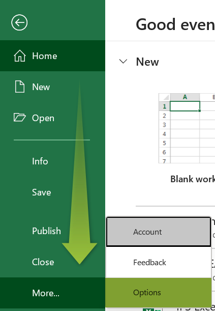
But first, to access the FTEST Excel feature from Data → Data Analysis, we must install the Excel add-in, Analysis ToolPak, to get the Data Analysis option in the Data tab.
For example, the Data tab ribbon does not show the Data Analysis feature.

So, the steps to show the Data Analysis feature in the Data tab are as follows:
- Select File from the top menu and then Options.

The Excel Options window opens.
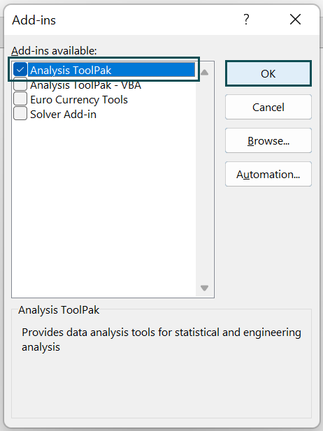
- Pick the Add-ins option, set the Manage field as Excel Add-ins, select the Analysis ToolPak option in the inactive applications list, and click Go.

- The Add-ins window will open, where we need to pick the Analysis ToolPak option and click OK.

The above steps will make the Data Analysis feature visible in the Data tab.


We can now click the Data Analysis option to access the Data Analysis window and apply the FTEST Excel feature.
Let us continue with the above example to see the steps to apply the FTEST Excel feature using Data Analysis.

Suppose we must perform the one-tailed F-Test for the given arrays and display the output in cell F2. Then, the steps are:
- Step 1: Choose Data Analysis from the Data tab.
- Step 2: Pick the required F-Test option in the Data Analysis window.
- Step 3: Set the below settings for applying the FTEST function.
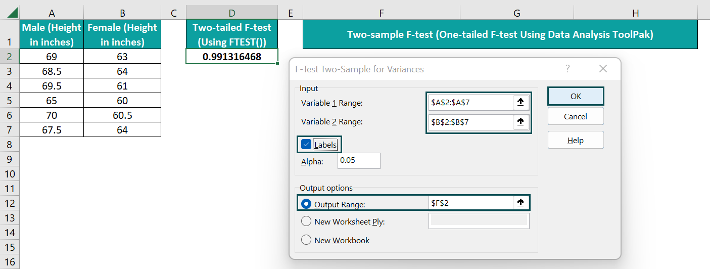
The two array ranges include the column names in the Input section fields. So, select the Labels option to show the array columns’ names in the output and set the Alpha value as 0.05, the significance threshold. And, as we need to output in the current sheet in cell F2, set the required Output options settings as shown above.
- Step 4: Click OK to view the result.
Suppose the null hypothesis is that the two arrays have the same variances. Then, the one-tailed F-Test Excel interpretation is that the p-value is 0.49 and greater than 0.05, the Alpha value. Also, the F-value, 1.0102, is less than the F Critical value, 5.0503. So, we can not reject the null hypothesis. And, thus chances are that the two given arrays have similar variances.
Examples
Check out the below examples to ensure we use the FTEST Excel function effectively.
Example #1
The table below shows the results of Tests 1 and 2 in seconds.

Suppose the requirement is to determine the two-tailed probability of the variances of the two tests not to be considerably different and show the result in cell B9. Then here is how we can apply the FTEST Excel function in the target cell and achieve the required output.
- Step 1: Select the target cell B9, enter the following FTEST Excel function, and press Enter.
=FTEST(A2:A7,B2:B7)
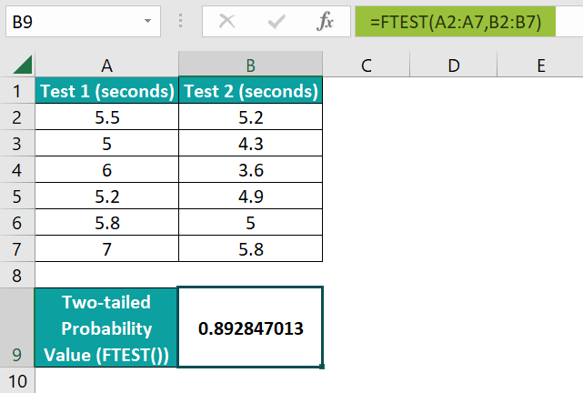
The FTEST() accepts the two array ranges, Test 1 and 2, as the input and returns the two-tailed probability of their variances not being significantly different as 0.8928. As this value is greater than 0.05, the significance threshold, we can not reject the null hypothesis, thus proving the variances to be almost the same.
Example #2
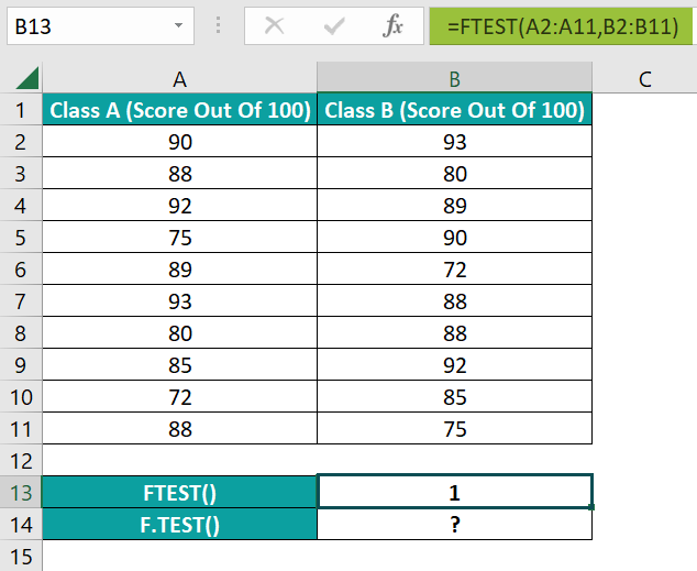
The following table shows the scores secured in two classes.
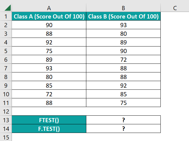
Suppose we must calculate the two-tailed probability of the variances of the two score sample sets not being significantly distinct. Then, using the FTEST Excel function can help us achieve the required probability value.
We shall see how the FTEST Excel function and its improved version F.TEST(), work. Assume the target cells are B13:B14.
- Step 1: Select the target cell B13, enter the FTEST(), and press Enter.
=FTEST(A2:A11,B2:B11)
- Step 2: Select the target cell B14, enter the F.TEST(), and press Enter.
=F.TEST(A2:A11,B2:B11)
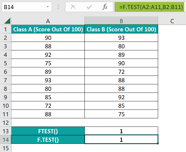
We can either directly enter the F.TEST() in the target cell or apply it by selecting the required cell and navigating the path Formulas → More Functions → Statistical → F.TEST.
Both FTEST Excel function and F.TEST() accept the two given arrays as the two argument values to return the required probability value as 1. It implies that the two score sample sets have equal variances.
Example #3
The table below shows two sample sets of ages.
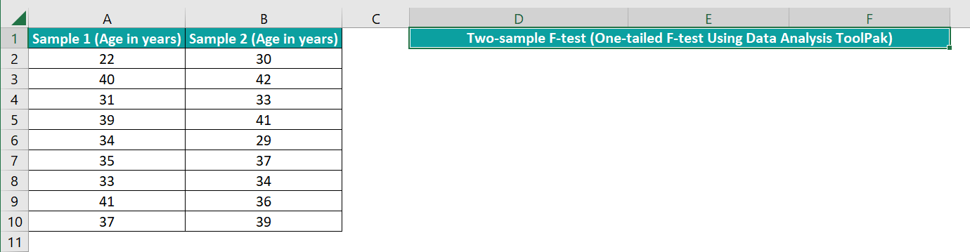
Suppose the requirement is to conduct the one-tailed F-Test, with the null hypothesis being that the two data sets have the same variance. And the alternate hypothesis is that Sample 1 has a higher variance than Sample 2. Assume the target cell is D2.
Then, here is how we can apply the FTEST Excel feature from the Data Analysis option in the Data tab.
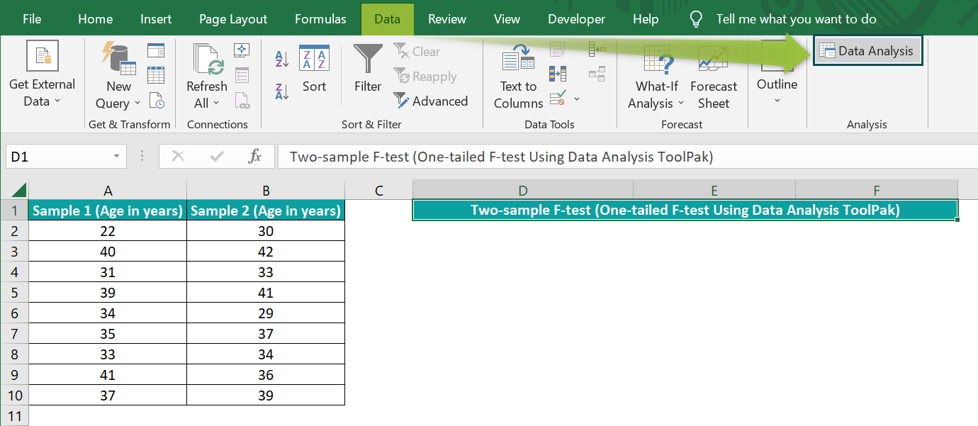
- Step 1: Click Data → Data Analysis to open the Data Analysis window.
- Step 2: Pick the option to perform the one-tailed F-Test in the Data Analysis window and click OK.

- Step 3: The corresponding window opens, where we must enter the two given array ranges, the significance threshold (Alpha) value, and the target cell address.
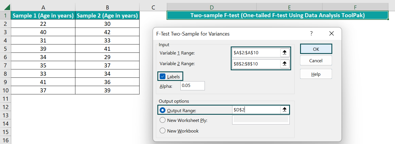
- Step 4: Click OK to view the result as a one-tailed F-Test Excel template depicted below.
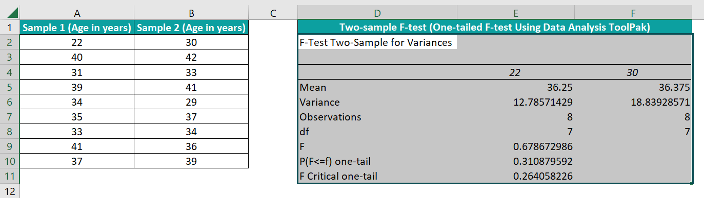
The above one-tailed F-Test Excel template shows the mean values and variances of the two samples in the cell range E5:F5 and E6:F6. We can observe that the variances are not significantly different.
Cells in the range E7:F7 show each data set’s total count of the data points. And the parameter df indicates the degree of freedom, which is one less than the Observations.
The F-value is the ratio of the larger and smaller samples’ variances.

where,
- σ1² : The larger sample’s variance.
- σ2² : The smaller sample’s variance.
In this example, the datasets have the same size. So, dividing the determined variances of the two datasets, 33.75 and 21, gives 1.607142857.
On the other hand, the determined p-value is 0.258660693, a value greater than the significance threshold value of 0.05. And the F-value is less than the F Critical. So, we cannot reject the null hypothesis, which is in line with our observation.
FTEST Excel Errors
Below are the scenarios when we can face FTEST Excel errors.
- Suppose one of the two arrays contains less than 2 data points or has a 0 variance. Then, the FTEST Excel function returns the #DIV/0! error.
- The FTEST() ignores text values, logical values, and blank cells but counts 0. However, if the two arrays contain only such values, the FTEST function returns the #DIV/0! error.
Important Things To Note
- Ensure to supply the FTEST Excel function arguments as numbers, arrays, names, or references to cell ranges containing the specified numbers.
- For arrays containing less than 2 data points or having 0 variances, the FTEST() output is the #DIV/0! error.
- If the supplied arrays do not contain numbers and only include values such as text, logical values, blank cells, or 0, the FTEST function output will be the #DIV/0! error.
Frequently Asked Questions (FAQs)
The FTEST function in Excel is in the Formulas Tab. Click Formulas → More Functions → Compatibility → FTEST to access the function.
However, if we require to use the latest function F.TEST(), go to Formulas → More Functions → Statistical → F.TEST to apply it in the required cell.
We can use the FTEST Excel function for two arrays of different sizes in the following way.
1. First, ensure the two given datasets contain valid data points.
2. Next, choose the required target cell and enter the FTEST(), specifying the two arrays of different sizes as the function arguments.
3. Finally, press Enter to view the calculated probability value.
Let us see the steps with an example.
The below table contains two datasets of weight values. While the first array contains six data points, the second includes five.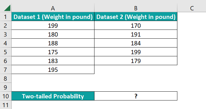
Suppose the requirement is to determine the two-tailed probability of the two given data sets’ variances not being significantly different and show the output in cell B10. Then, the steps to apply the FTEST() in the target cell and get the required probability value are as follows:
• Step 1: Select the target cell B10, enter the FTEST(), and press Enter.
=FTEST(A2:A7,B2:B6)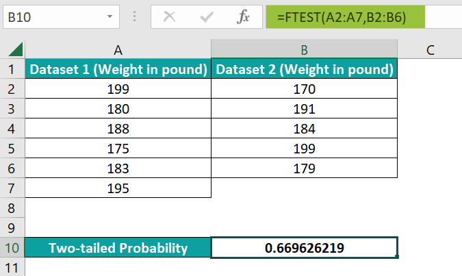
The FTEST() accepts the two given arrays of different sizes (cell ranges A2:A7 and B2:B6) and returns the probability of their variances not being considerably different as 0.669626219.
The Excel FTEST function return value of 1 means that the two given arrays have the same variance.
Use this FTEST Excel Template to follow along with the examples in this article.
Download Excel Template