What Is HLOOKUP In Google Sheets?
The HLOOKUP in Google Sheets is an inbuilt LOOKUP function. It looks for a value in the first row of the source dataset. It then returns a value in the same column from the cited row holding potential return values. The function is helpful when dealing with data provided in rows instead of columns.
Users can utilize the HLOOKUP function in Google Sheets for extracting information from massive datasets, merging data from different sources, and reviewing lists for discrepancies.
For example, the source dataset contains monthly headcount data of a team at a firm and the resource onboarding dates.

We must find the team headcount for April, cited in cell B5. Assume the target cell is B6.
Then, adhering to the definition of HLOOKUP in Google Sheets explained earlier, we can use the HLOOKUP() in the target cell to fetch the required result. Please note that this function works like the Excel HLOOKUP function.

The HLOOKUP() accepts four input values. The first argument, search_key, is the reference to the cell B5 holding the month Apr we must search.
Next, the second argument, range, value is B1:G3, where the function must search the search_key in the topmost row of the range. The third argument, index, value is 3 since we must find the corresponding return value from the third row of the range. Finally, the last argument, is_sorted, value is 0, indicating that the function must find an exact match for the search_key.
So, the function finds an exact match for the month Apr in cell E1 of the first row of the range B1:G3. Thus, the HLOOKUP In Google Sheets returns the cell E3 (where column E and row 3 of the range B1:G3 meet) value, 55, as the required output.
Table of contents
Key Takeaways
- The function HLOOKUP in Google Sheets looks for the search key in the topmost row of the cited search range for a match based on the specified match type. It then returns the value in the same column of the row, cited as the row range containing the potential return values.
- The HLOOKUP function in Google Sheets is useful for extracting data row-wise in massive datasets based on an exact or approximate match.
- We can apply the HLOOKUP function in Google Sheets as a standalone function. However, nesting it and using it with the VLOOKUP function and wildcard characters yield practical results.
HLOOKUP() Google Sheets Formula
The HLOOKUP function in Google Sheets syntax is the following:
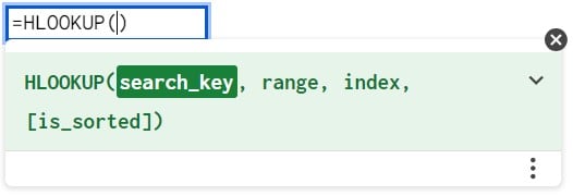
Where,
- search_key: The value we aim to look for.
- range: It is the search range, where the topmost row is searched for the search_key.
- index: The index of the row from where the value should be returned while considering the first row in the range as the number 1 row. When the index argument value is not within 1 and the number of rows in the range, the function will return the #VALUE! error.
- is_sorted: The argument value denotes whether the values in the topmost row of the cited range the function should search are sorted.
- When the argument value is the default value of TRUE or omitted, the function output is the closest match, which is below or equal to the search_key. However, if all the values in the search row exceed the search_key, the HLOOKUP In Google Sheets returns the #N/A error.
- Assume the argument value is the default value of TRUE or omitted. However, the values in the first row of the cited range are not in sorted order. Then, it is most likely that HLOOKUP() returns an incorrect value.
- When the argument value is FALSE, the function checks for an exact match for the search_key to return the required target value. However, in the case of multiple matching values, the function returns the cell value corresponding to the first match. On the other hand, if the function does not find any such value, its output is the #N/A error.
Furthermore, please supply the first three arguments when using HLOOKUP In Google Sheets, as they are mandatory. However, the last argument value is optional.
How To Use HLOOKUP In Google Sheets?
We can utilize the HLOOKUP function in Google Sheetsin the following two ways:
- Access the function from the ribbon.
- Enter the function into the sheet manually.
Method #1 – Access The Function From The Ribbon
Select a cell for displaying the output value – The Insert tab – The Function optionright arrow- The Lookup function group right arrow – The HLOOKUP function.
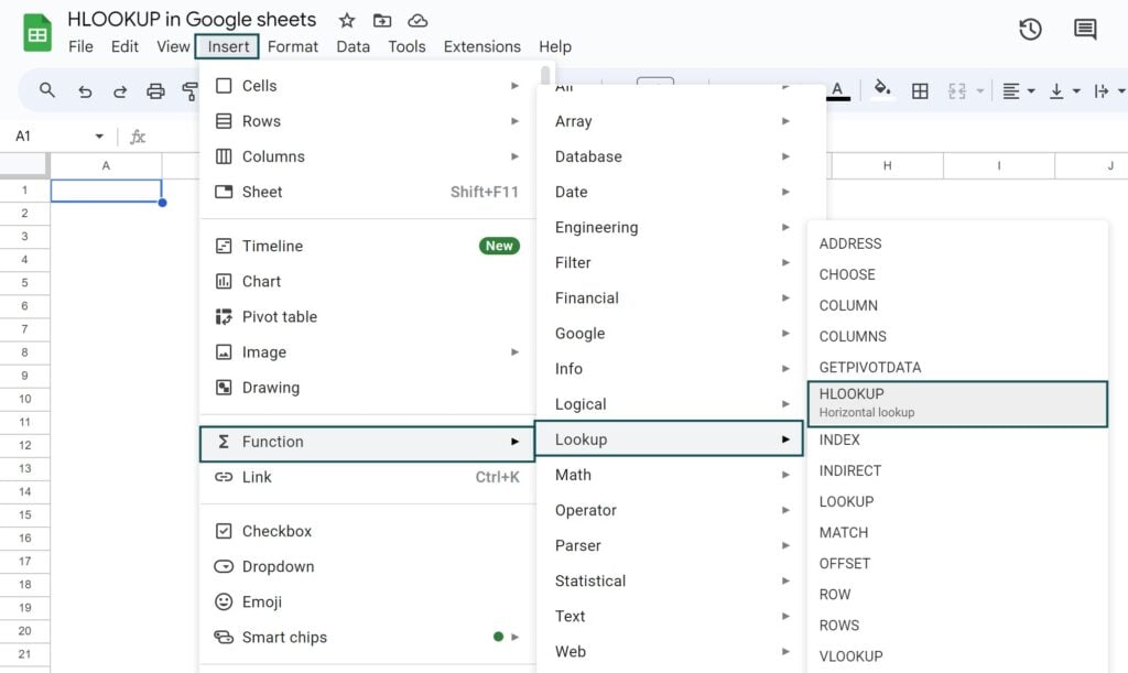
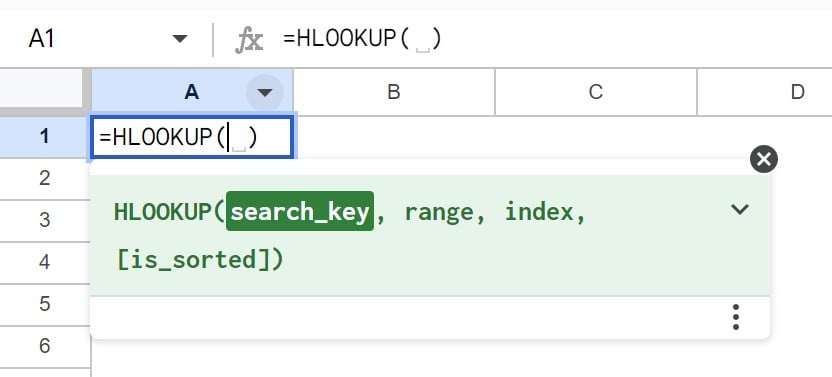
The chosen function will appear in the target cell, with the cursor inside the function brackets. We can now update the HLOOKUP in Google Sheets arguments within the brackets.

Moreover, we can click the ‘?’ symbol next to the function name to view its syntax.
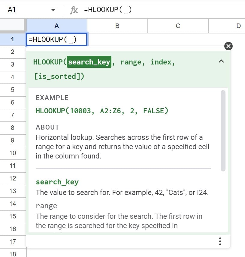
Next, select the down arrow in the syntax window to view the meaning of the function HLOOKUP In Google Sheets explained with an example.
Finally, once we enter the HLOOKUP in Google Sheets arguments, separated by commas, press Enter to view the function return value.
Method #2 – Enter The Function Into The Sheet Manually
- Select the cell where we aim to show the result.
- Type =HLOOKUP( in the cell. [ Alternatively, type =H or =HL and click the function name HLOOKUP from the listed options to choose the function.]
- Feed the argument values, separated by commas, and close the brackets.
- Press Enter to fetch the HLOOKUP() output.
Examples
The illustrations below describe the practical ways of using HLOOKUP in Google Sheets.
Example #1 – Nested HLOOKUP
The first source dataset lists employees, their designations and monthly salaries. The second dataset holds the appraisal status for each designation.
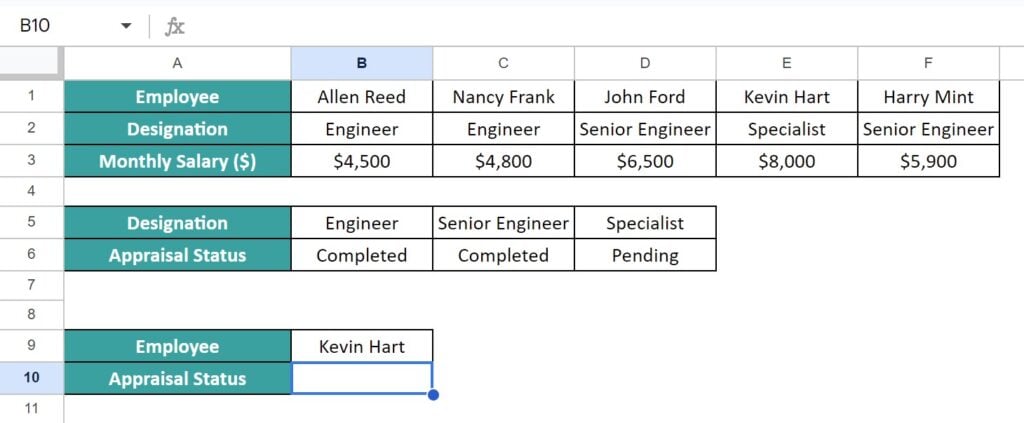
The task is to determine the appraisal status of the employee cited in cell B9. Assume the target cell is B10.
Then, we can use the nested HLOOKUP() in the target cell to secure the required result.
Step 1: Select the target cell B10 and enter the nested HLOOKUP().
=HLOOKUP(

[ Alternatively, select the target cell and then Insert à Function à Lookup à HLOOKUP function.


The above step will insert the function in the required cell.]
Step 2: Update the function arguments within the brackets.
=HLOOKUP(HLOOKUP(B9,B1:F3,2,0),B5:D6,2,0)


Step 3: Press Enter to view the nested HLOOKUP() output.

The inner HLOOKUP() searches the cited employee, Kevin Hart, for an exact match in the first row of the range B1:F3. It finds the match in cell E1. Thus, the function returns the employee Kevin Hart’s designation from the second row of column E in the range B1:F3, which is the cell E2 value, Specialist.
Next, the outer HLOOKUP() searches the determined designation Specialist for an exact match in the first row of the range B5:D6. It finds the match in cell D5. Thus, the function returns the employee Kevin Hart’s appraisal status from the second row of column D in the range B5:D6, which is the cell D6 value Pending.
Example #2 – HLOOKUP With VLOOKUP
The source dataset contains the quarterly inventory-level data for various branch offices of a firm.

We must update the Q3 inventory level for the branch office, cited in cell H1. We shall consider cell H3 as the target cell.
Step 1: Choose the target cell H3, enter the VLOOKUP() containing the HLOOKUP(), and press Enter.
=VLOOKUP(H1,$A$2:$E$9,HLOOKUP(H2,$A$2:$E$9,2,0),0)

The cell range B3:E3 in the source dataset holds the indices of the columns containing the quarterly inventory levels, with the indices starting from 2.
The VLOOKUP(), that works like the Excel VLOOKUP function, accepts four inputs. The first argument, search_key, value is the reference to the cell H1 value, Madison. Next, the second argument, range, value is the lookup range A2:E9.
The third argument, index, is the HLOOKUP(). The HLOOKUP() accepts four argument values. The first argument, search_key, is the reference to the cell H2 value of Q3. Next, the second argument, range, value is the search range A2:E9. The third argument, index, value is 2, indicating that the function must return the value from the second row of the range A2:E9. Finally, the last argument, is_sorted, value is 0, denoting that the function must find the exact match for the search_key.
So, the HLOOKUP() finds an exact match for the search_key Q3 in the first row of the range A2:E9. It finds the exact match in cell D2. So, the function returns the value in the cell where column D and row 2 in the range A2:E9 meet, which is the cell D3 value of 4.
So, the VLOOKUP() considers the HLOOKUP() output value of 4 as the index of the column holding the potential return values, which is column D of the lookup range A2:E9. Next, the last argument, is_sorted, value is 0, indicating that the function must find the exact match for the search_key.
Thus, the VLOOKUP() looks for an exact match for the search_key Madison in the first column of the range A2:E9. It finds the exact match in cell A8, which is in row 7 of the lookup range A2:E9. So, the function returns the value in the cell where column D and row 7 in the range A2:E9 meet, which is the cell D8 value of 1200.
Example #3 – HLOOKUP With Approximate Match
The source dataset shows the bonus eligibility status based on specific revenue values.

The requirement is to determine the bonus eligibility status for the revenue value cited in cell B4. Assume the target cell is B5.
In this case, the revenue value of $1,900, specified in cell B4, is not in the list of revenue figures in the source dataset. So, we can find the approximate match for the specified revenue value of $1,900 using the HLOOKUP() in the target cell to get the corresponding detail.
Step 1: Select the target cell B5, enter the HLOOKUP(), and press Enter.
=HLOOKUP(B4,B1:G2,2)

The HLOOKUP() takes three inputs. The first argument, search_key, is the reference to the cell B4 holding the revenue value of $1,900 we must search.
Next, the second argument, range, value is B1:G2, where the function must look for the search_key in the topmost row of the range. The third argument, index, value is 2 since we must find the corresponding return value from the second row of the range. Finally, we ignore the last argument, is_sorted. So, the function takes the argument’s default value of 1,indicating that the function must find an approximate match for the search_key.
Further, the values in the search range are in ascending order. So, the function output is the closest match, which is less than or equal to the search_key.
So, the function finds an approximate match for the revenue value of $1,900 in cell E1 of the first row of the range B1:G2. Thus, the HLOOKUP() returns the cell E2 (where column E and row 2 of the range B1:G2 meet) value, Eligible, as the required output.
Drawbacks
The drawbacks of the HLOOKUP function in Google Sheets are as follows:
- When searching for the search key, the HLOOKUP() always searches the first row in the cited range argument value. We cannot search the search_key in rows below the first row.
- The HLOOKUP() is not dynamic. It implies that inserting a row in the cited search range will not update the index argument value automatically. So, we will need to update the new range and index argument values in the HLOOKUP formula manually.
Difference Between the HLOOKUP Google Sheets Function and VLOOKUP
The differences between the HLOOKUP Google Sheets function and the VLOOKUP function are as follows:
- Definition
The HLOOKUP() looks for the search value horizontally in the given source dataset. On the other hand, the VLOOKUP() searches for the value vertically in the given source dataset.
- Syntax
The HLOOKUP() in Google Sheets syntax is the following:

The VLOOKUP() in Google Sheets syntax is the following:

- Logic
The HLOOKUP() considers that the source dataset holds the data in different rows. On the other hand, the VLOOKUP() considers that the source dataset holds the data in different columns.
- Usage
The HLOOKUP() helps determine the data from a row, which can be anywhere below the topmost row of the source dataset. On the other hand, the VLOOKUP() helps determine the data from a column, which can be anywhere on the right of the leftmost column of the source dataset.
Important Things To Note
- Assume that the HLOOKUP in Google Sheets cannot locate the search key, and the is_sorted argument value is TRUE. Then, the function locates the largest value that is below or equal to the search key to return the target value, provided the values in the first row of the search range are sorted.
- When the search key is less than the least value in the first row of the specified range, the HLOOKUP function in Google Sheets output is the #N/A error value.
- When the cited is_sorted argument value is FALSE, and the search key is a text value, we can utilize the wildcard characters “?” and “*” in the search_key argument value.
Frequently Asked Questions (FAQs)
We can use Wildcards in the HLOOKUP function in Google Sheets, as shown below with an example.
The source dataset shows a list of teams and the units of stocks they sold. Please note that each team name starts with a unique character.
We need to update the stocks sold by the team specified in cell B4. Assume the target cell is B5.
Then, we can use the HLOOKUP() with the wildcard character, ‘*’, in the target cell to secure the required count.
Step 1: Select the target cell B5, enter the HLOOKUP(), and press Enter.
=HLOOKUP(“T*”,B1:F2,2,0)
We supply “T*” instead of the reference to the cell B4 holding the specific team name as the first argument to the HLOOKUP(). The reason is that no two team names start with the same character. So, we can specify the first character of the team name, followed by the wildcard character ‘*’, as the search key.
Next, the second argument is the search range B1:F2, where the function must search for the search key in the topmost row of the range. The third argument value is 2, indicating that the function must fetch the return value from the second row of the specified search range. Finally, the last argument value of 0 denotes that the function must find an exact match for the search key.
So, the function looks for the team name starting with the character “T” in the first row of the search range B1:F2. The function finds an exact match in cell E1. So, it returns the value in the cell where column E and row 2 meet, which is the cell E2 value of 400 as the required output.
The HLOOKUP doesn’t work in Google Sheets due to the following reasons:
• The supplied range argument value does not include the row from where we aim to obtain the return value.
• The supplied range value does not include the row where we must search the search key, or the search row is not the topmost row in the specified range.
• The search key is not present in the source dataset. However, we enter FALSE or as the is_sorted argument value in the HLOOKUP().
• Assume that we add or remove one or more rows to or from the search range. Then, the existing index argument value makes the formula return an incorrect value.
We can perform error handling in HLOOKUP in Google Sheets by nesting the HLOOKUP() within the IFERROR function. The formula will help in displaying an appropriate comment instead of the error the HLOOKUP() returns.
Download Template
This article must be helpful to understand the HLOOKUP In Google Sheets, with its formula and examples. You can download the template here to use it instantly.
Recommended Articles
Guide to What Is HLOOKUP In Google Sheets. Here we explain how to use HLOOKUP function in Google Sheets with examples and points to remember. You can learn more from the following articles –

Leave a Reply