VLOOKUP Wildcard in Google Sheets

What Is VLOOKUP Wildcard in Google Sheets?

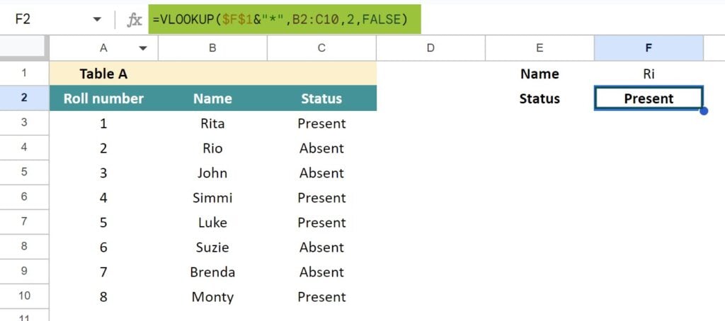
If you have datasets on your spreadsheet, VLOOKUP helps you search for related information by row. When working with data, finding information across multiple sheets is very difficult. Thus, with VLOOKUP Wildcard in Google Sheets, we can look up and retrieve matching data from another table, either in the same sheet or a different sheet. For instance, we have some student roll numbers, names, and their status. We have to find if a student with a name beginning with “Ri” is present/absent. Enter the following formula in cell F2.

=VLOOKUP($F$1&”*”,B2:C10,2,false)

The above formula looks for the first instance of the student’s name beginning with “Ri” and gives the corresponding output from the second column of the range, i.e., present.

Google Sheets VLOOKUP SYNTAX

As you must have seen in the example above, the VLOOKUP does a vertical lookup by searching for the specified value in the first column of the given range. It then returns a value from the same row of another column. Hence, the VLOOKUP function can be written as follows.

VLOOKUP(search_key, given range, index, [is_sorted])

• Search_key – this is the value we search for
• Range – the data range for the search. The first column of the range is searched for the search_key in this case.
• Index – the column number in the range from which a matching value should be returned(first column’s index is 1, 2nd column is 2 and so on).
• Is_sorted – indicates whether the lookup column is sorted (TRUE) or not (FALSE). The default is TRUE.

Notes:

1. If the fourth value is specified as TRUE, the first column must be in ascending order.
2. If is_sorted is FALSE, the first column does not have to be sorted.

How to VLOOKUP Wildcard (*,?) in Google Sheets?

#1 – Typical VLOOKUP Function

VLOOKUP in Google Sheets helps you look up related information by row while looking up a value in a vertical column. However, in most cases, the lookup table might be on different sheets. Let us look at an example in which we retrieve the value from a different sheet. When you access a range in a table from another sheet, you write the range as follows: Sheet2!A3:B10.

 Let us look at an example to understand this better. 

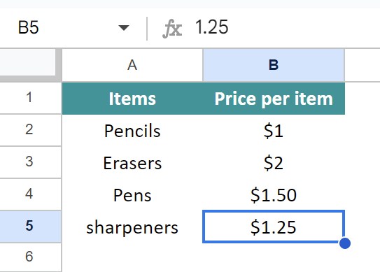
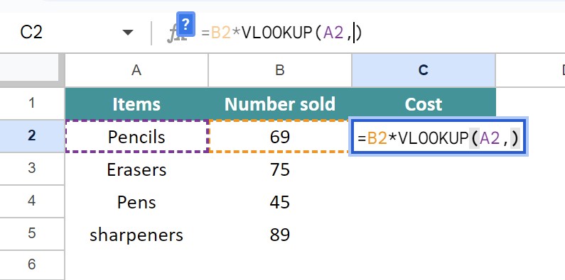
The images show tables from two sheets. The first sheet contains details of some items and the number sold. The second sheet contains the cost of each item.

Sheet 4

Sheet 3

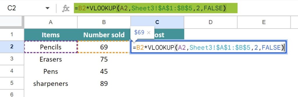
Step 1: Let us apply the VLOOKUP function. Here, we must search for each item on the first sheet with the corresponding unit cost on the second sheet. Enter the following formula in cell C2. First, let us look at the search value. In this case, it is “Pencils.”

=VLOOKUP(A2,

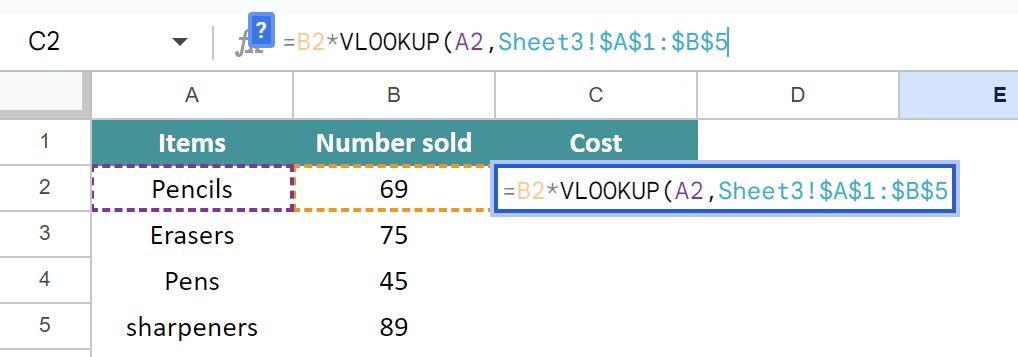
Step 2: Next is the crucial step where we must specify the range. Since the range is in Sheet3 while we are in sheet 2, we enter the range as follows.

=VLOOKUP(A2, Sheet3!A1:B5,

Step 3:  The last two arguments are the index of the column to be looked up and the value TRUE/FALSE, depending on whether the data is sorted. Since we are finding the cost of the number of items sold, the final formula is as follows.

=B2*VLOOKUP(A2,Sheet3!A1:B5,2,FALSE)

Step 4: Press Enter. You get the cost price of 69 pieces of the item sold(at $1 per piece).

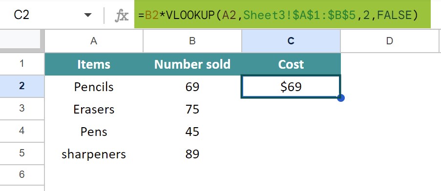
Step 5: Drag the Autofill handle to get the cost of other items sold. Before that, we fixed the reference of the range, so it does not change as Sheet3!$A$1:$B$5.

#2 – Asterisk (*)

Example #1

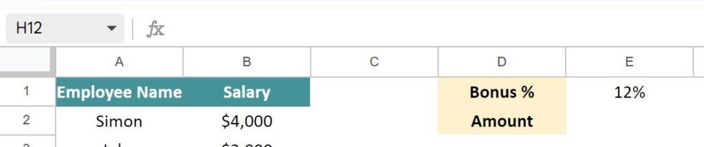
Let us now look at the VLOOKUP Wildcard in Google sheets (similar to excel VLOOKUP wildcard). There is a table in the given sheet. It contains the details of the employee, like name and salary. Calculate the bonus amount received by employees whose name begins with a particular letter.

Let us set out to find the bonus of an employee whose name begins with the letter A if present in the data set. He is to be given a bonus of 10%, entered in cell E1.

Step 1: Let us suppose you want to find the bonus amount against the salary of an employee beginning with the letter A.

1. The first argument would be “A*”
2. The next argument would be the range where we would look up this value. Hence, it is A1:B8.
3. The third argument includes the column index, where we will retrieve the value from the same row.
4. The fourth argument is FALSE, as the data is not sorted.

Since we are calculating the bonus with the given percentage for the retrieved value, let us enter the following formula in E2.

=E1*VLOOKUP(“A*”,A1:B8,2,FALSE)

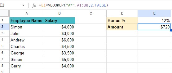
Step 2: Press Enter, and you get the bonus amount of the person whose name starts with A.

Step 3: Let us change A* to C* and check the results.

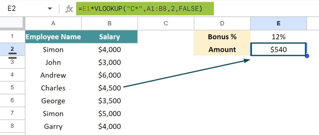
You can observe how the bonus amount changes from “Andrew” to “Charles.”

Example #2

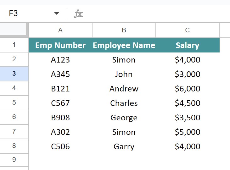
As seen in the above example, we have used the value to be found directly in the formula. We can use the formula to search for a particular salary. Let us alter the example. We add another column before the employee name and give it the employee number.

Step 1: Now, let us look at an employee whose employee number begins with A. Three numbers are beginning with A. Enter the following formula in cell F2.

Step 2: We get the bonus amount of the first occurrence of the employee whose employee number begins with A3, which is John in this case.

#3 – Question Mark (?)

As seen earlier, the * is used to match a sequence of characters while Question mark (?) is used to match any single character, while looking up values. In other words, a question mark matches any single character.

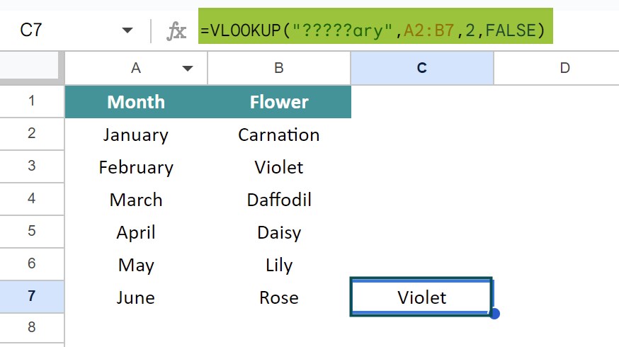
In the example below, we have some flowers and the birth month they represent. Let us look up these flowers using a ? (question mark) and the VLOOKUP function.

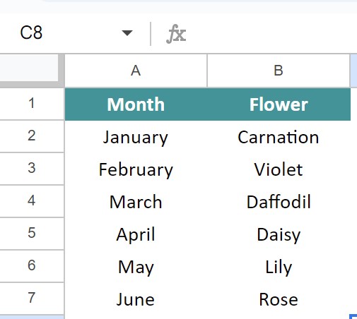
Step 1: To apply the VLOOKUP wildcard in Google Sheets,  we will try to find the flower representing February. Apply the following formula in cell C7.

=VLOOKUP(“?????ary”,A2:B7,2,FALSE).

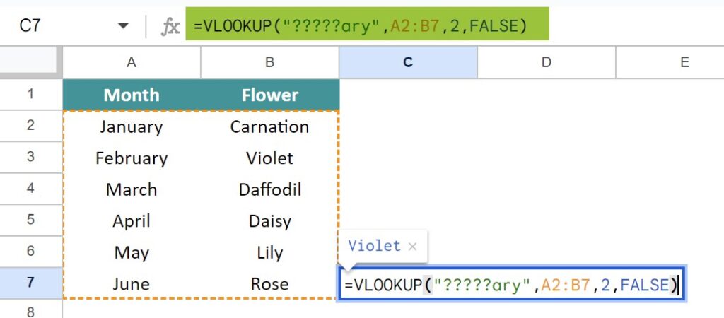
Step 2: As observed, we have given the search value as ?????ary. There are two months that end in “ary.” How does VLOOKUP distinguish between the two?

It is based on the number of ‘?.’ While January has just four letters before “ary,” February has five letters, and hence, since there are 5 ?, it returns the flower corresponding to February.

Important Things to Note

1. Remember that VLOOKUP is not case-sensitive. It does not distinguish between lower and uppercase letters.
2. VLOOKUP Wildcards in Google Sheets always search in the first column of the range.
3. If VLOOKUP wildcard Google Sheets return wrong values, set the fourth argument to FALSE to return exact matches.
4. VLOOKUP can search using wildcard characters like the asterisk (*) and question mark (?).
5. As the VLOOKUP function cannot look to its left, for such scenarios, you may use the VLOOKUP in conjunction with INDEX MATCH.
6. The MERGE Sheets add-on in Google Sheets allows you to search without effortlessly using the formula.
7. If you mistakenly specify a range that is bigger than the maximum number of columns in the range, you get a #REF error.

Frequently Asked Questions (FAQs)

Download Template

This article must be helpful to understand the VLOOKUP Wildcard in Google Sheets, with its formula and examples. You can download the template here to use it instantly.

Recommended Articles

Guide to What Is VLOOKUP Wildcard in Google Sheets. We explain how to use VLOOKUP Wildcard in Google Sheets with examples. You can learn more from the following articles. –

• VLOOKUP Two Criteria In Google Sheets
• VLOOKUP Names In Google Sheet
• SUMIF With VLOOKUP In Google Sheets