SUMIF With VLOOKUP In Google Sheets

What Is SUMIF With VLOOKUP In Google Sheets?

The SUMIF with VLOOKUP in Google Sheets is a SUMIF formula, with the VLOOKUP() supplied as its dynamic criterion argument. The VLOOKUP() helps retrieve the return value for the specified lookup value to ensure the SUMIF() totals the rows of data based on the return value cited as the criterion.

Users can use the SUMIF with VLOOKUP formula in Google Sheets when the lookup value, given as a criterion, is in another dataset. The other dataset can be in the same or different sheet as the main table containing the values to add conditionally.

For example, we have two datasets. The first is the main one containing the sales representative IDs and their date-wise sales-generated data. On the other hand the second is a lookup table, which lists the sales representatives and their IDs.

We must determine the total sales generated by the sales representative, cited in cell F9, and display the output in cell F10. Also, since the target cell must show a currency value, it has the same data type format as cells C2:C11.

Then, we can apply the SUMIF(), with the VLOOKUP() as its second argument, in the target cell to secure the required outcome. The logic will be inline with the meaning of SUMIF with VLOOKUP In Google Sheets explained earlier.

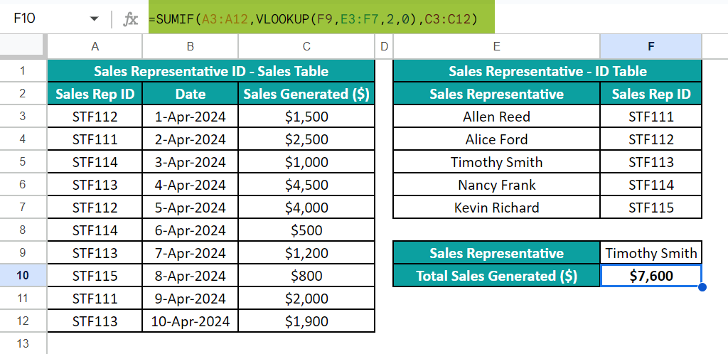
We must add the column C sales values pertaining to the sales representative Timothy Smith. So, we can search the representative’s name in the first dataset to add the applicable sales values using the SUMIF().

However, the main table lists the representatives’ IDs instead of their names, with the sales representatives’ names and IDs provided in another table. So, we achieve the output by using SUMIF with VLOOKUP in Google Sheets formula, which works with the similar logic as SUMIF with VLOOKUP in Excel.

Furthermore, the SUMIF() and the VLOOKUP() individually work as the Excel SUMIF function and Excel VLOOKUP function.

The SUMIF() accepts three inputs, with the second argument, criterion, being the VLOOKUP().

First, the VLOOKUP() looks for the sales representative name in the second dataset. Since it finds a match in cell E5, the function returns the corresponding ID in the cell in the 5^th row of column F, which is the cell F5 value, STF113.

So now, the SUMIF() tests the condition, which is the VLOOKUP() output value of STF113 in the range A3:A12. It finds the matches in cells A6, A9, and A12. Next, the function adds the sales values in rows 6, 9, and 12 of column C, which are the cells C6, C9, and C12 values.

Thus, the formula SUMIF with VLOOKUP in Google Sheets returns $7,600 as the required total sales generated by the specified sales representative.

Syntax

The SUMIF-VLOOKUP formula in Google Sheets syntax is the following:

Where,

• range: The range that we need to test against the condition, which in this case is the VLOOKUP() output.
• VLOOKUP(): The function output is the criterion argument value. It is the condition that the SUMIF() checks for in the range. The VLOOKUP function arguments are the following:
  • search_key: The value to search for in the first column of the lookup range.
  • range: The top and bottom limits of the lookup range.
  • index: The index of the column in the specified range containing the return value. Also, it is a positive number.
  • is_sorted: The value denotes whether the VLOOKUP() should look for an exact or approximate match.
    • FALSE (0): The recommended value representing an exact match search.
    • TRUE (1): It represents an approximate match search. The function considers it as the default value if we ignore the argument.

Also, in the scenario of an approximate match, the lookup value range should be sorted in ascending order. Otherwise, the function output may be incorrect.

• sum_range: The range containing the values to add based on the given condition if it is different from the specified range.

Furthermore, we must supply all the argument values when using SUMIF with VLOOKUP in Google Sheets, except for the last ones in the two functions, as they are optional.

How To Use SUMIF With VLOOKUP In Google Sheets?

The steps to apply the SUMIF with VLOOKUP formula in Google Sheets are as follows:

1. Choose the cell where we aim to display the result.
2. Type =SUMIF( in the cell. [ Alternatively, type =S or =SU and click the function name SUMIF from the listed options to select it.]
3. Supply the first argument and enter a comma. Next, type VLOOKUP(. Otherwise, type V or VL and click the function name VLOOKUP from the listed options to select it.) After that, supply the VLOOKUP() argument values, separated by commas, and close the bracket. Finally, enter a comma and the SUMIF()’s last argument to update the SUMIF With VLOOKUP In Google Sheets arguments, and close the bracket.
4. Press Enter to acquire the formula output.

Examples

The following examples describe the practical ways of using the SUMIF-VLOOKUP formula, adhering to the concept of SUMIF With VLOOKUP In Google Sheets explained earlier.

Example #1 – Use Of SUMIF(VLOOKUP) Together To Determine Some Value

The main table shows the product codes and their store-wise inventory level data.

We need the total inventory level of the product, cited in cell F8, to show the value in cell F9.

The issue is that we can not look up the product name in the main table to determine the required total inventory level of the specific product. The reason is that the first table lists product codes and not the names. However, we have a separate lookup table mapping the product names and their codes.

In such a case, we can implement the SUMIF-VLOOKUP formula in the target cell to secure the desired outcome.

Step 1: Select the target cell F9 and enter the SUMIF().

=SUMIF(

Enter the first argument, range, value, which is A3:A13, followed by a comma.

The second argument is the criterion, which is the VLOOKUP(). So, enter the function name and the opening bracket.

Now, enter the first argument, search_key, value in the VLOOKUP(), which is cell F8, followed by a comma.

The next argument in the function is the range, which is the lookup range of E3:F6, and enter a comma.

After that, we must supply the third argument, index, value. In this case, we need the VLOOKUP() to return the product ID. So, the argument value is 2.

Next, enter a comma and as we must find an exact match, enter the fourth argument, is_sorted, value as 0. Close the bracket and enter a comma.

Finally, we will enter the last argument, sum_range, in the SUMIF(), which is the range holding the inventory level data, C3:C13. So, now we have entered all the SUMIF with VLOOKUP In Google Sheets arguments. Next, close the bracket to complete the formula.

=SUMIF(A3:A13,VLOOKUP(F8,E3:F6,2,0),C3:C13)

Step 2: Press Enter to execute the SUMIF-VLOOKUP formula in the chosen cell.

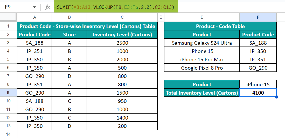
First, the VLOOKUP() looks for the product iPhone 15, in the range E3:F6. It finds the exact match in cell E4. So, the function returns the value in the cell where row 4 and column F intersect, which is the cell F4 value, IP_350.

Next, the SUMIF() searches for the product code IP_350, which the VLOOKUP() returned as the condition in the range A3:A13. The function locates the exact matches in cells A5, A6, A12, and A13. So, the function adds the inventory level values in the cells in the corresponding rows of column C since the specified sum_range is C3:C13. So, the function adds the cells C5, C6, C12, and C13 values and the SUMIF With VLOOKUP In Google Sheets returns 4100 as the total inventory level of the product specified in cell F8.

Example #2 – Determining Sum Based On Matching Criteria In Different Work Sheets

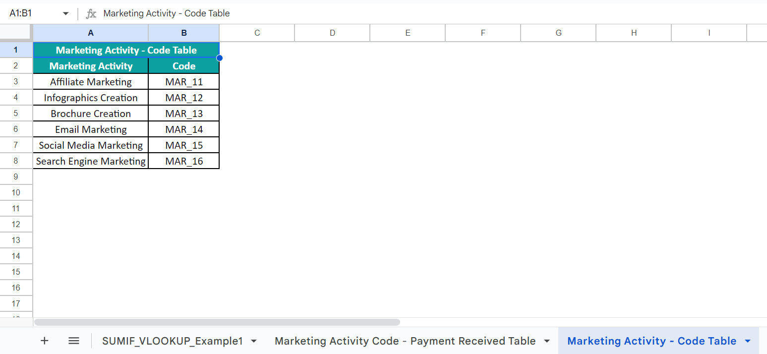
Consider that we have two sheets. While the first one contains the source dataset, the second contains the lookup table.

The source dataset in the first sheet lists the marketing activity codes, and the corresponding date-wise payment received data. On the other hand, the lookup table in the second sheet contains the list of marketing activities and their codes.

The requirement is to determine the total payment received for the marketing activity specified in cell F1 and show the output in cell F2 in the first sheet. Please note the target cell data type is the same as the range C3:C12, Currency.

Then, the steps to implement the SUMIF-VLOOKUP function in the target cell to secure the anticipated result are as follows:

Step 1: Choose cell F2 and enter the SUMIF().

=SUMIF(

Enter the first argument value, A3:A12, followed by a comma.

Next, enter the VLOOKUP() as the criterion argument value.

We will enter the first argument in the VLOOKUP(), which is the search key, the cell reference to the value in cell F1, followed by a comma.

The second argument in the VLOOKUP() is the range, which is in the second sheet. So, click the second sheet tab to open the second sheet and choose the range A3:B8 as the lookup range.

Next, enter a comma.

After that, supply the third argument, index, value. In this case, we need the VLOOKUP() to return the marketing activity code. So, the argument value is 2.

Next, enter a comma and since we should find an exact match, enter the fourth argument, is_sorted, value as 0. Close the bracket and enter a comma.

After that, we shall enter the last argument, sum_range, in the SUMIF(), which is the range containing the payment received data, C3:C12. Finally, close the bracket.

=SUMIF(A3:A12,VLOOKUP(F1,’Marketing Activity – Code Table’!A3:B8,2,0),C3:C12)

Step 2: Press Enter to implement the SUMIF-VLOOKUP formula in the selected cell.

First, the VLOOKUP() searches for the marketing activity, Infographics Creation, in the range A3:B8. It locates the exact match in cell A4. So, the function returns the value in the cell where row 4 and column B meet, which is the cell B4 value, MAR_12.

Next, the SUMIF() looks for the marketing activity code MAR_12 in the range A3:A12, which the VLOOKUP() returned as the criterion. The function finds the exact matches in cells A3, A7, and A10. So, the function adds the payment received values in the cells in the corresponding rows of column C since the specified sum range is C3:C12. Thus, the function adds the cells C3, C7, and C10 values to return $1,350 as the total payment received for the marketing activity specified in cell F1.

Important Things To Note

• The SUMIF and VLOOKUP functions in the SUMIF with VLOOKUP in Google Sheetsformula are not case sensitive.
• Assume the VLOOKUP() in the SUMIF-VLOOKUP formula does not find a match for the lookup value. Then, the VLOOKUP() returns the #N/A error, and the SUMIF-VLOOKUP formula output will be 0. Also, if the criterion specified in the SUMIF() is not met, the SUMIF-VLOOKUP formula returns 0 as the output.
• Assume the sum_range argument range holds only non-numeric values. Then, the SUMIF-VLOOKUP formula returns 0 as the output.

Frequently Asked Questions (FAQs)

Download Template

This article must be helpful to understand SUMIF With VLOOKUP In Google Sheets, with its formula and examples. You can download the template here to use it instantly.

Recommended Articles

Guide to What Is SUMIF With VLOOKUP In Google Sheets. We explain how to use the formula in Google Sheets with examples & points to remember. You can learn more from the following articles. –

• VLOOKUP With MATCH In Google Sheets
• Data Validation In Google Sheets
• IFERROR In Google Sheets