What Is Match Data in Excel?
Match data in Excel is a method to check each cell in a column against the corresponding cell in another column to identify a match. On the other hand, if the values in the cells we compare do not match, we can display an appropriate message.
Users can utilize the match data method in Excel while performing risk assessments and cost estimations using data in one or more spreadsheets.
📥Download the ready-to-use Excel template to practice this tutorial yourself.
How To Match Data In ExcelFor example, the image below shows two datasets.
The first lists students and their test scores in Mathematics in descending order of the scores. On the other hand, the second lists the same students, but in alphabetical order, and their test scores.
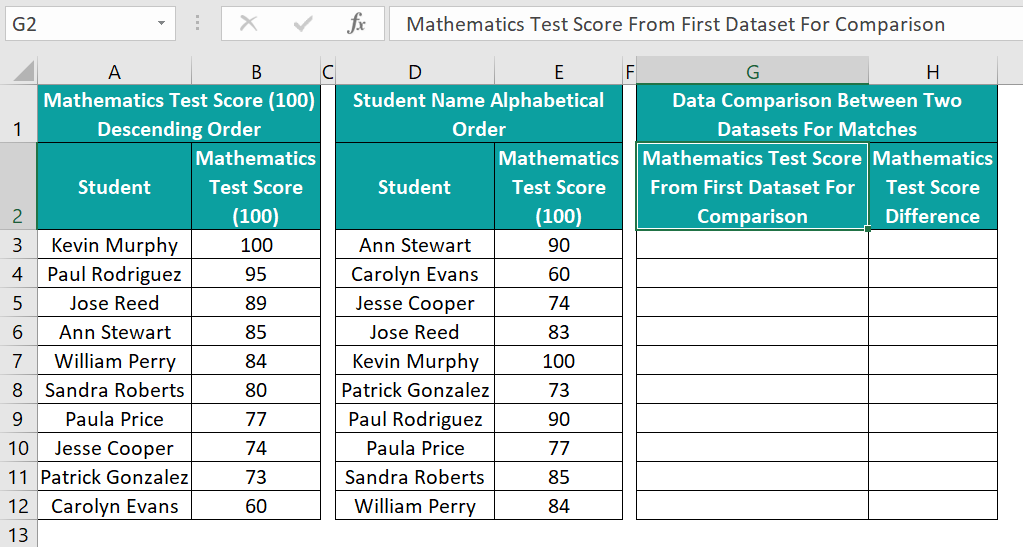
The aim is to check if each student’s score is the same in the two datasets and show the difference in the test scores of each student, if any, in column H.
Then, we can find and match data in Excel in columns G and H, using the Excel VLOOKUP function and the Subtraction operator, ‘–‘, respectively.

In the above find and match data in Excel example, we apply the VLOOKUP() in column G since the student names are in different orders in the two datasets. The function updates the test score of each student, specified in the second dataset, based on the first dataset.
Next, we find the difference between the test scores in each row of columns E and G. This step helps us determine the students for whom the test scores match in the two datasets.
A difference of 0 between two test scores indicates a match. On the other hand, if the difference is a non-zero value, it indicates a mismatch between the test scores in the two datasets.
Furthermore, the above method will also work when the two datasets are in two different sheets, and we must match data in Excel from 2 worksheets.
Table of contents
Key Takeaways
- The match data in Excelis a technique to check if the value in a cell in one column matches the value in the corresponding cell in another column. The columns can be on the same or different sheets. Also, we can display customized messages for matches and discrepancies.
- Users can match data in one or more sheets to find matching data and differences in the data in different datasets while working with financial and accounting data.
- Users can use the VLOOKUP(), INDEX + MATCH function and use these functions based on uniquely-created lookup values to match data in one or more worksheets.
How To Match Data In Excel?
We can match data in a spreadsheet using the following methods:
- Match Data Using VLOOKUP Function
- Match Data Using INDEX + MATCH Function
- Create Your Own Lookup Value
Method #1 – Match Data Using VLOOKUP Function
The steps to compare and match data in Excel using the VLOOKUP function and the Subtraction operator, ‘–‘, are as follows:
- Choose a cell to apply the VLOOKUP().
- Enter the following VLOOKUP() formula in the chosen cell.
=VLOOKUP(lookup_value_dataset2, table_array_dataset1, col_index_num, [range_lookup])
While the lookup value will be in the second dataset, the table array will be in the first dataset. On the other hand, the col_index_num and range_lookup arguments have the same definition as in a regular VLOOKUP().
- Press Enter to view the required return value corresponding to the specified lookup value.
- Choose a cell to check if the data in the second dataset and the VLOOKUP() return value in the corresponding row match or not.
- Enter the ‘–‘- based formula to match data in Excel in the target cell, which determines if the required data in the two datasets match or are different.
=data_second dataset – data_VLOOKUP() return value
Thus, the VLOOKUP() helps obtain the data pertaining to the lookup value in the second dataset based on the first. Next, the second formula helps determine the data match and mismatch between the two datasets.
Method #2 – Match Data Using INDEX + MATCH Function
This method is helpful when the target column containing the return value we aim to retrieve is on the left of the range containing the lookup value.
The steps to compare and match data in Excel using the INDEX + MATCH function and the Subtraction operator, ‘–‘, are as follows:
- Choose a cell to insert the INDEX + MATCH function.
- Enter the following INDEX + MATCH () formula in the chosen cell.
=INDEX(array_dataset1,MATCH(lookup_value_dataset2,lookup_array_dataset1,[match_type]))
The array range in the INDEX Excel function will be in the first dataset, and the Excel MATCH function is the row_num argument value in the INDEX().
Next, while the lookup value will be in the second dataset, the lookup array will be in the first dataset in the MATCH(). On the other hand, the match_type argument has the same definition as in a regular MATCH().
- Press Enter to view the required return value corresponding to the specified lookup value.
- Choose a cell to check if the data in the second dataset and the INDEX + MATCH function return value in the corresponding row match or not.
- Enter the ‘–‘- based formula to match data in Excel in the target cell, which determines if the required data in the two datasets match or are different.
=data_dataset2 – data_ INDEX + MATCH_function_return value
Thus, MATCH() returns the position of a cell in the first dataset as the required row number based on the lookup value in the second dataset. Next, the INDEX() finds the value of the cell in the first dataset at the intersection of the specified column and row number the MATCH() returns. Next, the second formula helps determine the data match and mismatch between the two datasets.
Method #3 – Create Your Own Lookup Value
Sometimes, the lookup value in the second dataset may appear multiple times in the lookup range in the first dataset.
Then, the VLOOKUP and the INDEX + MATCH functions output will be the return value corresponding to the first appearance of the lookup value in the first dataset. But in some cases, this output may be incorrect.
Thus, here is how to create unique lookup values for the two datasets in question to obtain the correct return value for every lookup value.
- Insert a new column in the first dataset, and the new column must be before the column containing the target values we aim to find based on the lookup values.
- Concatenate the first dataset values in each row of the newly inserted column to form unique lookup values using the ‘&’ symbol, CONCAT(), or Excel CONCATENATE function.
- Insert a new column in the second dataset and repeat step 2 using the second dataset’s values to create unique lookup values.
- Apply method #1 or #2 to match data in a worksheet based on the newly created unique lookup values.
Please note that all three methods discussed above will work when we must match data in Excel from 2 worksheets.
Examples
Check out the following match values in Excel examples to use the functionality effectively.
Example #1 – Match Data Using VLOOKUP Function
We have a dataset containing a list of products and their order quantities, updated in two files manually, and they are as depicted in the image below.
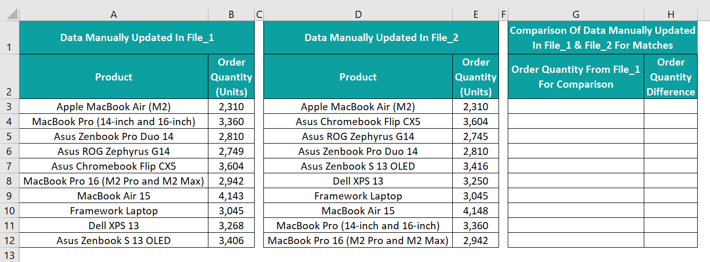
The task is to compare and match the order quantity data for each product in the two datasets. Assume the target columns are G and H.
Then, here is how to use the VLOOKUP() in column G to find the order quantity values for the products listed in File_2 based on the File_1 dataset. Then, use ‘–‘ in column H to find the difference between the order quantity value in File_2 and the VLOOKUP() output for each product to find the required matches.
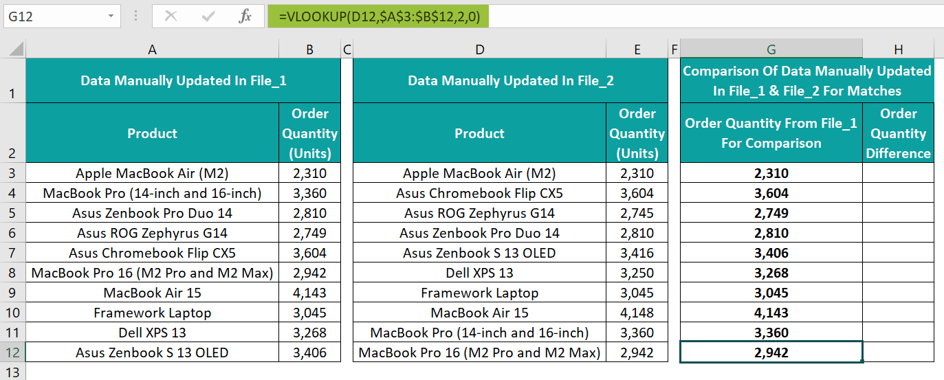
- Step 1: Choose cell G3, enter the VLOOKUP(), and press Enter.
=VLOOKUP(D3,$A$3:$B$12,2,0)

- Step 2: Using the Excel fill handle, update the VLOOKUP() in cells G4:G12.
- Step 3: Choose cell H3, enter the below formula, and press Enter.
=IF((E3-G3)=0,”-“,(E3-G3))
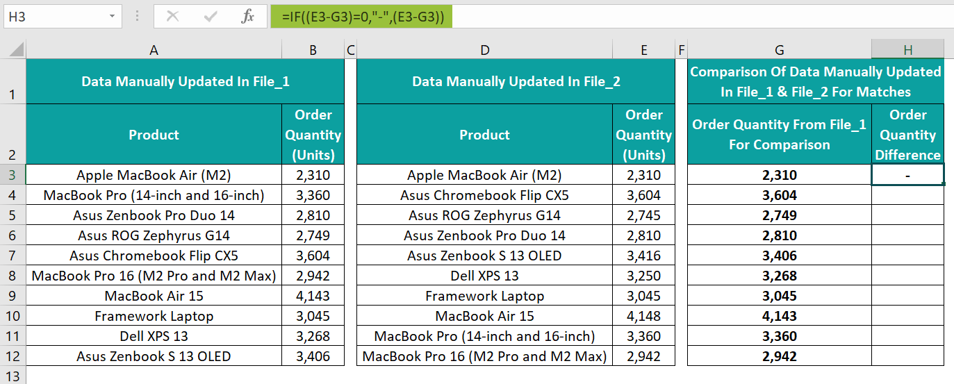
- Step 4: Using the Excel fill handle, update the formula in cells H4:H12.
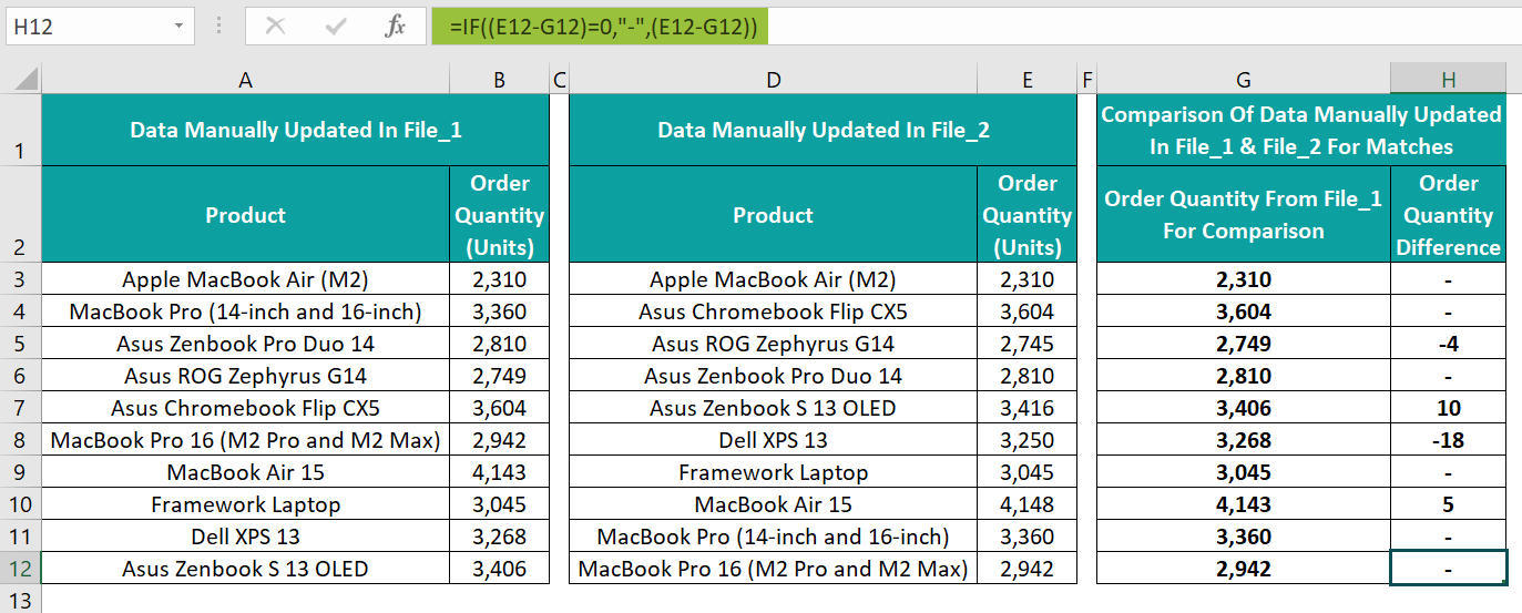
Let us check the row 12 formulas in cells G12 and H12 to understand the method and the output.
The VLOOKUP() in cell G12 searches for the cell D12 lookup value in the range A3:B12 and returns the corresponding return value from the range B3:B12, 2,942.
Next, the Excel IF function condition contains the subtraction formula, which finds the difference between the order quantity value in cell E12 and the VLOOKUP() output in cell G2. The IF() condition checks if the difference equals zero. Since the condition holds in this case, the IF() returns the TRUE value, ‘–‘, indicating the order quantity values in the two files for the product cited in File_2 match.
Thus, in this way, we can find the matches between two datasets and also the discrepancies to correct them.
Example #2 – Match Data Using INDEX + MATCH Function
The image below shows two datasets containing the monthly sales figures at a firm.
However, while the first dataset follows month-wise order, the second is the corresponding months in each quarter-based.
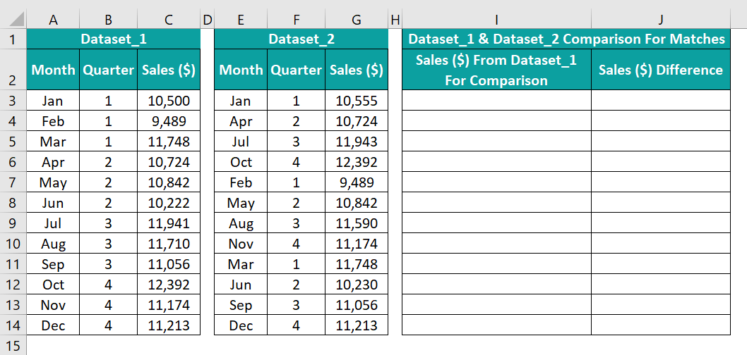
Thus, since the data order differs in the two datasets, the requirement is to compare the sales figures in the two datasets for the matches and differences. Assume the target columns as I and J.
Then, we can use the INDEX + MATCH function in column I cells and the ‘–‘ sign in column J cells to achieve the required match and difference data.
- Step 1: Choose cell I3, enter the INDEX + MATCH function, and press Enter.
=INDEX($C$3:$C$14,MATCH(E3,$A$3:$A$14,0))

- Step 2: Using the Excel fill handle, update the INDEX + MATCH function in cells I4:I14.
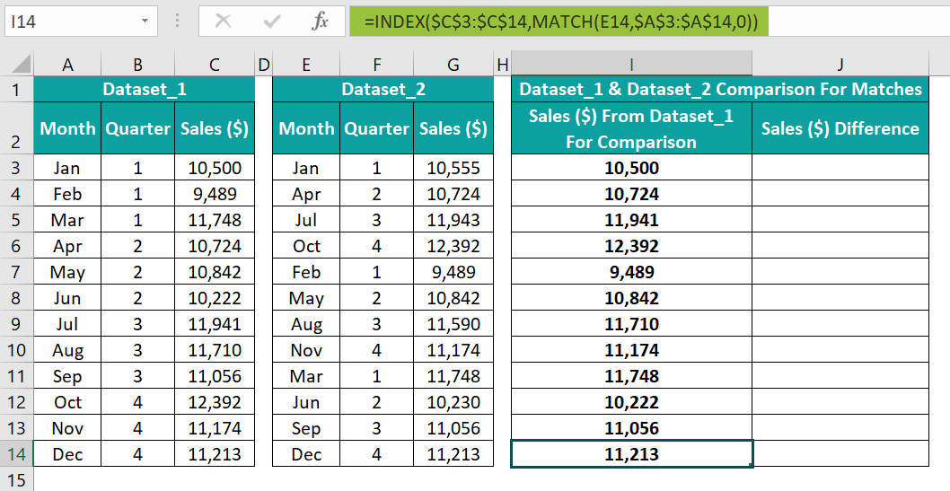
- Step 3: Choose cell J3, enter the below formula, and press Enter.
=IF((G3-I3)=0,”-“,(G3-I3))
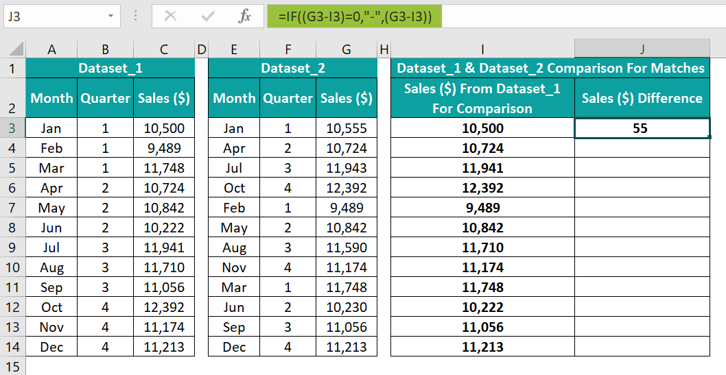
- Step 4: Using the Excel fill handle, update the formula in cells J4:J14.
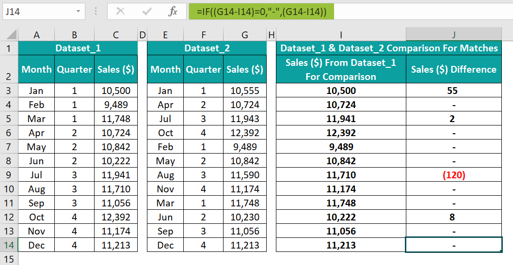
Let us check the row 14 formulas in cells I14 and J14 to understand the method and the output.
The MATCH() in cell I14 finds the position of the lookup value, “Dec”, in the range A3:A14, which is 12. Next, the INDEX() determines the value in the cell at the intersection of the 12th row of column range C3:C14 and the column range C3:C14, which is cell C14 value, 11,213.
Next, the subtraction formula in the IF() condition finds the difference between the sales figure in the second dataset in cell G14 and the INDEX + MATCH function output in cell I14. Since the difference is 0, the IF() condition holds, leading to the IF() returning the TRUE value, ‘–‘, indicating the December sales figures in the two datasets match.
Thus, the method helps find the matches between two datasets and also the discrepancies to resolve them.
Example #3 – Create Your Own Lookup Value
The image below shows two datasets containing a list of employees, their teams and annual salary details.
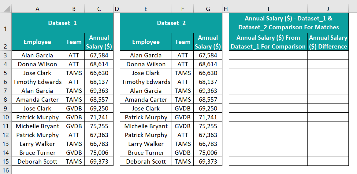
The task is to compare the annual salary data for each employee in the two datasets for matches.
Then, the steps are as follows:
- Step 1: Choose cell I3, enter the VLOOKUP(), and press Enter.
=VLOOKUP(E3,$A$3:$C$15,3,0)

- Step 2: Using the Excel fill handle, update the VLOOKUP() in cells I4:I15.

- Step 3: Choose cell J3, enter the below formula, and press Enter.
=IF((G3-I3)=0,”-“,(G3-I3))
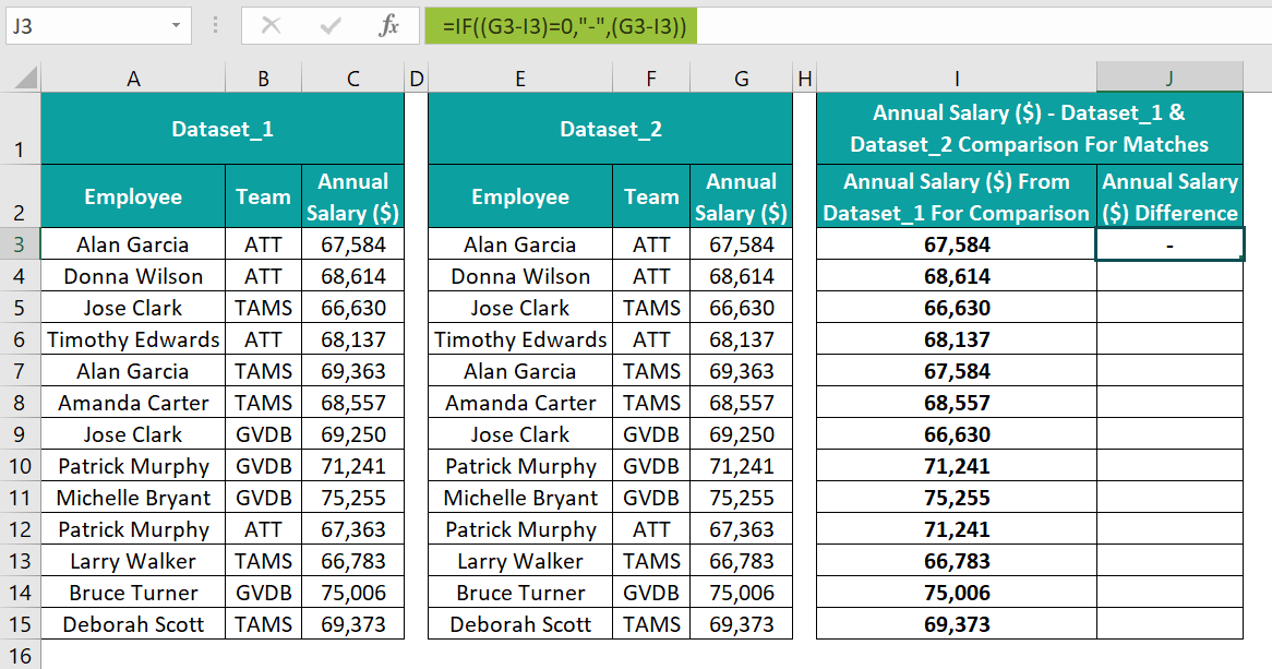
- Step 4: Using the Excel fill handle, update the formula in cells J4:J15.
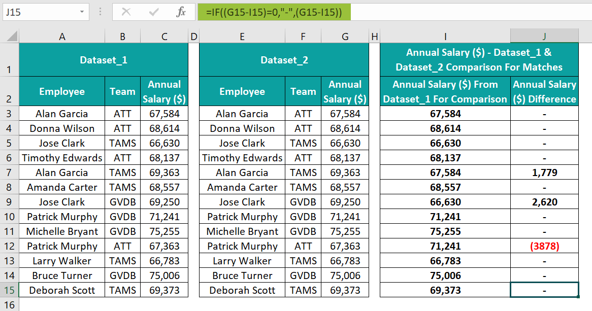
The output shows the annual salary figures for three employees, Alan Gracia, Jose Clark, and Patrick Murphy, do not match within the two datasets.
The reason is that the abovementioned names appear more than once in the lookup range. Hence, the VLOOKUP() output is the return value corresponding to the specific employee name’s first appearance in the lookup range, which may be incorrect.
So, here is how to create a unique lookup value for each employee to ensure the VLOOKUP() returns the correct output and required data matches for all the employees.
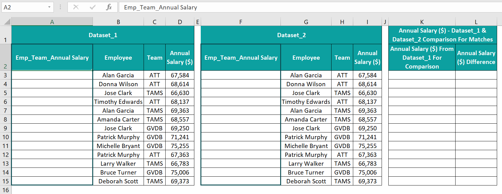
- Step 1: Introduce a new column in each dataset to update the unique lookup value for each employee.
Please ensure the new column in the first dataset is on the left of the target column containing the return value. Otherwise, the VLOOKUP() will not work.
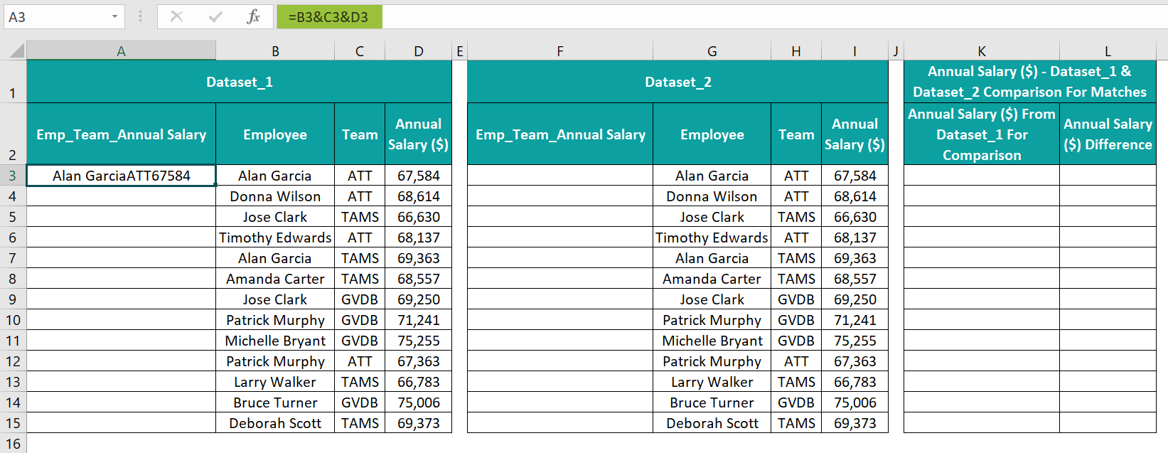
- Step 2: Choose cell A3, enter the following formula, and press Enter.
=B3&C3&D3
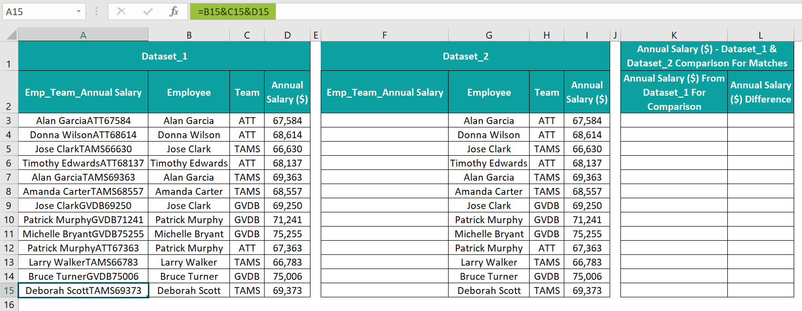
- Step 3: Using the fill handle, enter the formula in cells A4:A15.
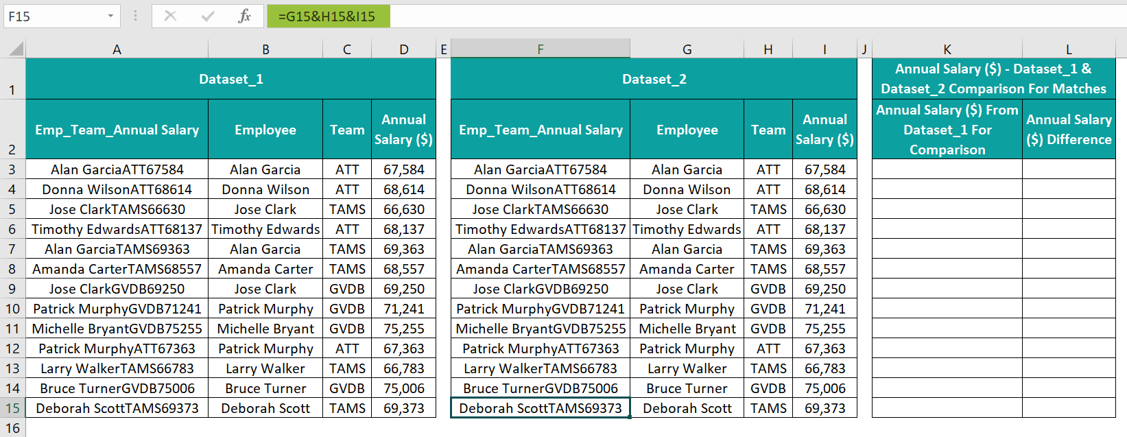
- Step 4: Choose cell F3, enter the below formula, and press Enter.
=G3&H3&I3

Step 5: Using the fill handle, enter the formula in cells F4:F15.
- Step 6: Choose cell K3, enter the VLOOKUP(), and press Enter.
=VLOOKUP(F3,$A$3:$D$15,4,0)
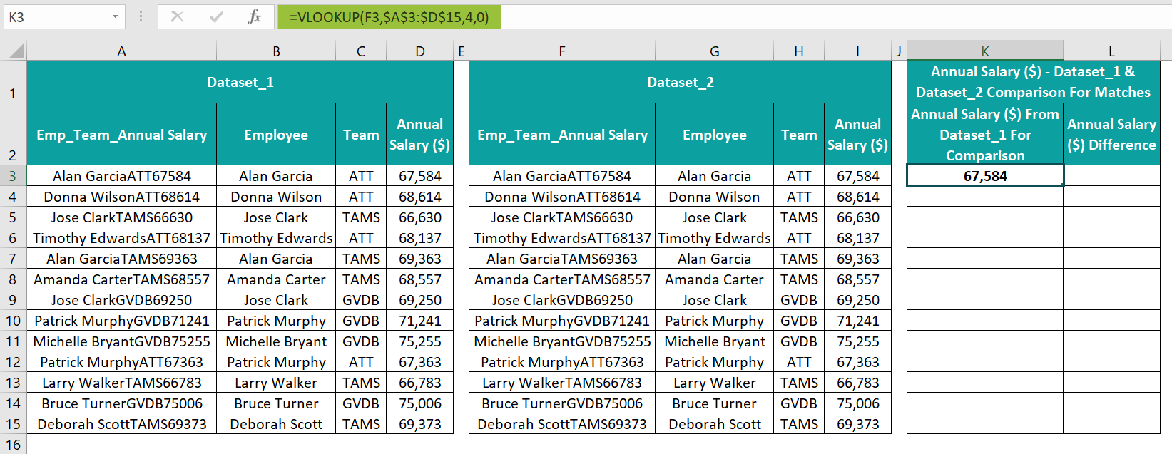
- Step 7: Using the fill handle, update the VLOOKUP() in cells K4:K15.
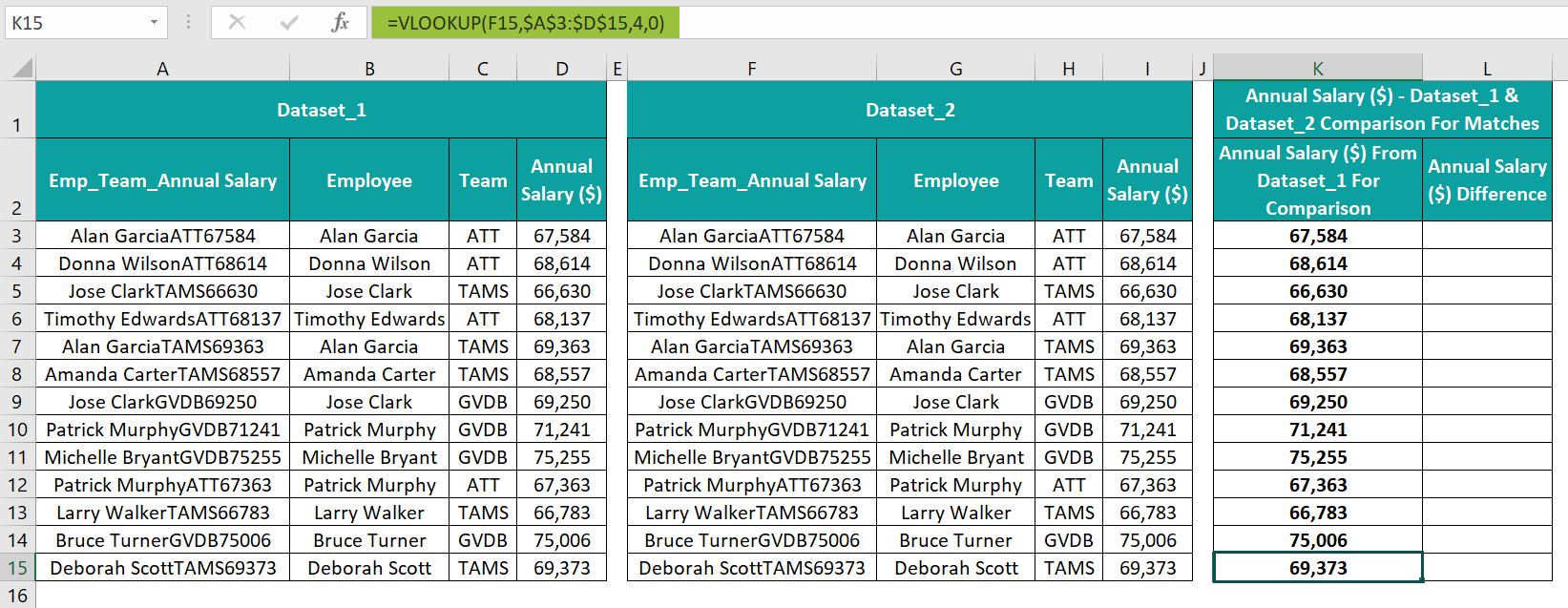
- Step 8: Choose cell L3, enter the IF(), and press Enter.
=IF((I3-K3)=0,”-“,(I3-K3))
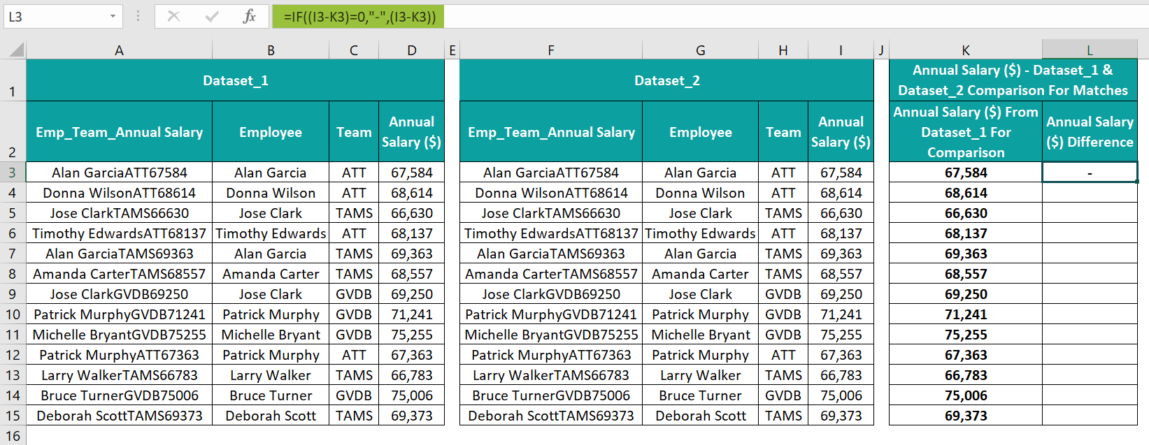
- Step 9: Using the fill handle, implement the formula in cells L4:L15.

The logic of this method is the same as Method #1, except the function will search the column F lookup value in column A and return the correct output accordingly.
Thus, now we see the discrepancies in the annual salaries of the three previously-mentioned employees are resolved. The reason is that the concatenated values used as the unique lookup values contain the employee name, their team and annual salary data. It leads to the VLOOKUP() locating the lookup value in the lookup range correctly and returning the corresponding return value.
Important Things To Note
- The argument values supplied to the VLOOKUP() to match data in Excel must adhere to the function syntax and definition. Otherwise, the function may return errors such as the #N/A, #REF!, Excel #VALUE! error, #NAME?, and #SPILL!.
- Switching the lookup and return column values and supplying invalid ranges to the INDEX + MATCH function to match Excel data can lead to incorrect output or errors.

Frequently Asked Questions (FAQs)
We can match data in Excel from 2 worksheets, as explained below with an example.
The first two images show two worksheets containing US states and their population statistics.

While the first worksheet shows the US states and population data by rank, the second contains the data in the alphabetical order of the US states.
The task is to compare the population data between the two sheets for matches. Assume the target cells are in the first sheet.
• Step 1: Choose cell D3 in the first worksheet and enter the VLOOKUP().
=VLOOKUP(A3,
Next, click the second worksheet tab to open it and select the lookup range A3:B17.
Excel will show the worksheet name of the chosen range in the formula.
After that, complete the VLOOKUP().
=VLOOKUP(A3,’US_State_Pop_Alphabetical Order’!A3:B17,2,0)
• Step 2: Press Enter to execute the function, and the first worksheet will open and show the function output in cell D3.
Next, make the range reference in the formula absolute.
• Step 3: Using the fill handle, update the formula in cells D4:D17.
• Step 4: Choose cell E3, enter the IF(), and press Enter.
=IF((B3-D3)=0,”-“,(B3-D3))
• Step 5: Using the fill handle, implement the formula in cells E4:E17.
The method’s logic is the same as that of Method #1, explained in the above article. However, the only difference is that the VLOOKUP() shows the worksheet name containing the lookup range, indicating that the match is between two worksheets.
We can match dates in Excel by first using any of the following formulas.
=cell_reference_date_value1=cell_reference_date_value2
Or
=VALUE(“cell_reference_date_value1”)=VALUE(“cell_reference_date_value2”)
Or
=VALUE(“valid_date_value1”)=VALUE(“valid_date_value2”)
Or
=DATEVALUE(“valid_date_value1”)=DATEVALUE(“valid_date_value2”)
You can match data in Excel with multiple criteria using the following array formula:
{=INDEX(return_range,MATCH(1,(criteria1=range1)*(criteria2=range2)*(…),0))}
While return_range is the range from which we aim the function to return the output or return value, criteria1, criteria2, … are the conditions for the match. And range1, range2, … are the ranges where the corresponding criteria should be checked.
Next, we can use the ‘–‘ operator to find the difference between the source dataset data and the corresponding INDEX-MATCH() output to determine if the values match or differ.
Download Template
📥Download the ready-to-use Excel template to practice this tutorial yourself.
How To Match Data In ExcelRecommended Articles
This has been a guide to How To Match Data In Excel. We learn to match data using VLOOKUP, INDEX + MATCH, & by creating our own lookup value, with examples. You can learn more from the following articles –

Leave a Reply