What Is Sum Multiple Excel Rows?
Sum multiple rows is a method to add the numeric data specified in two or more rows in Excel. The concerned rows can be in the same or different sheets in one or more workbooks.
Users can use the sum multiple Excel rows techniques to compute values such as the total revenue generated and units of inventory procured based on the provided raw data.
📥Download the ready-to-use Excel template to practice this tutorial yourself.
How-to-Sum-Multiple-Rows-in-Excel-TemplateFor example, the source dataset holds information regarding the sales generated by five sales representatives at a firm in 2023.
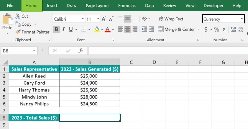
The aim is to determine the total sales generated in 2023 and display the output in cell B8, which has its data format set as Currency in the Number Format option in the Home tab.
Then, we can apply the formula to sum multiple rows in Excel cell B8 to secure the required total sales figure.
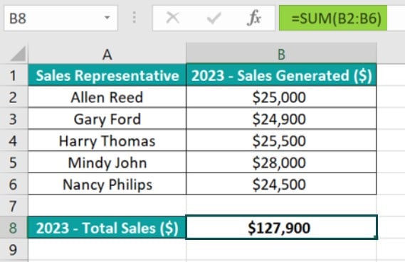
While we can sum multiple rows and columns in Excel, this example shows how we can add multiple rows in a worksheet.
We use the Excel SUM function in the target cell, with the input being the range of cells spanning across multiple rows and containing the individual sales figures we aim to add.
Next, once we enter the formula in the target cell and press Enter, the function returns the value of 127900. However, we set the target cell’s data format as Currency. Thus, the output appears as a currency value of $127,900.
Table of contents
Key Takeaways
- Sum multiple rows in Excel is a technique to total the required values specified in multiple rows across one or more sheets in one or multiple workbooks.
- We can use the SUM Excel function to add multiple rows of data. The input to the function can be the reference to the range of concerned rows, references to the cells in multiple rows, or directly the values in the specific rows.
- Users can sum multiple Excel rows when they must add finance or statistical data spread across two or more rows in massive datasets quickly.
How To Sum Multiple Excel Rows?
We can sum multiple rows in Excel utilizing the SUM function in the following ways:
- Access from the Excel ribbon.
- Enter into the worksheet manually.
Method #1 – Access From The Excel Ribbon
Select a cell for displaying the result – The Formulas tab – The Math & Trig group down arrow – The SUM function.
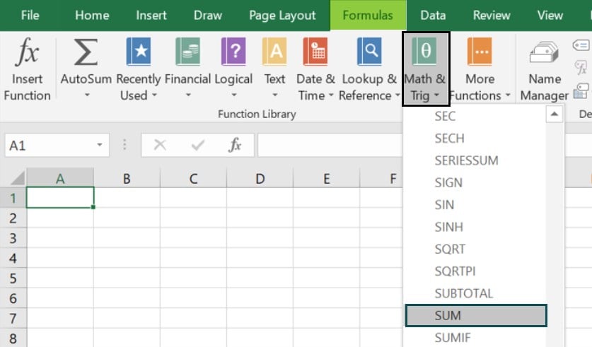
Once we choose the function, the Function Arguments window will appear. We can enter the values or the references to the rows or ranges of data we aim to add.
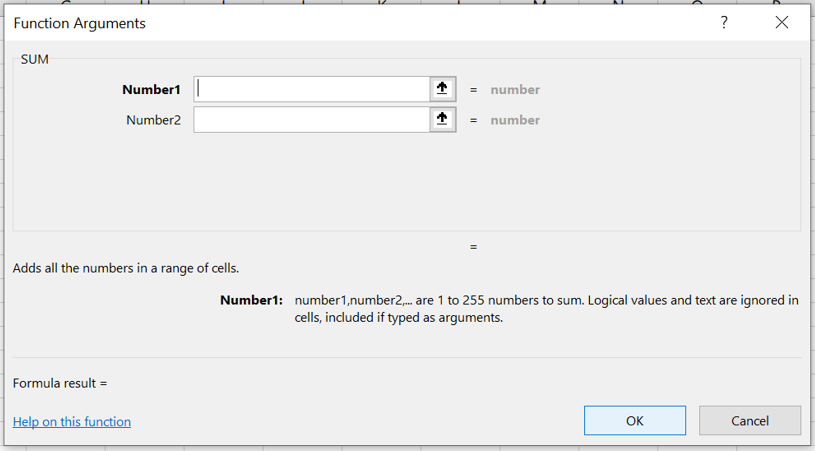
Finally, clicking OK will execute the formula to sum multiple rows in Excel.
Method #2 – Enter Into The Worksheet Manually
- Choose a cell to display the result.
- Type =SUM( in the cell. [Alternatively, type =S or =SU and double-click the SUM function from the options to select it.]
- Supply the arguments as values (separated by commas) or references to the concerned rows of data, and close the bracket.
- Press Enter to fetch the SUM function return value.
Furthermore, we can sum multiple rows in Excel based on criteria. In such a case, we can use inbuilt functions such as the Excel SUMIF function with multiple criteria and the Excel SUMIFS function.
On the other hand, the VLOOKUP sum multiple rows is another option available in Excel. It enables one to look up values corresponding to a search value and add the values to obtain the required sum value.
Examples
Though we can sum multiple rows in Excel based on criteria, the following examples explain the different ways to sum multiple Excel rows with no conditions involved.
Example #1 – Using SUM Function
The following dataset contains the date-wise inventory level at a store.

The task is to determine the total inventory level and display the output in cell B13.
In this case, we do not have to look up values associated with a specific search value. So, we do not need to resort to the VLOOKUP sum multiple rows option. Instead, we can directly add all the per-day inventory level figures using the SUM() in the target cell to acquire the required output.
Step 1: Choose cell B13, enter the SUM(), and press Enter.
=SUM(B2:B11)
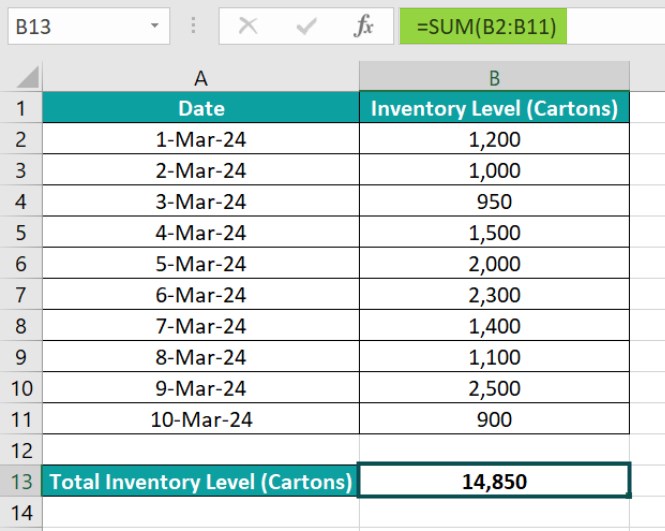
The per-day inventory level values are in cells across multiple rows, from rows 2 to 11. Thus, we can supply the reference to the cell range across rows 2 to 11 as the argument value to the SUM(). Otherwise, the inventory level figures or the Excel cell references to the cells holding the inventory level data in the concerned rows, separated by commas, can be the SUM() input.

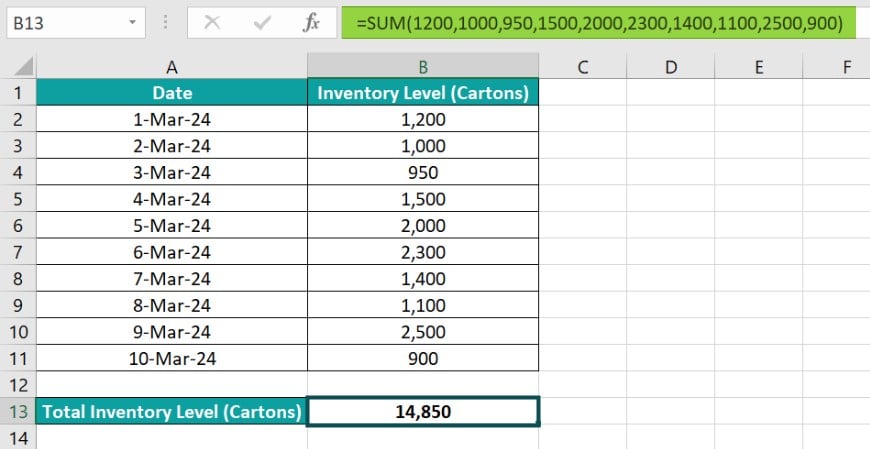
[Alternatively, choose the target cell and then Formulas – Math & Trig – SUM function.

The Function Arguments window for the function will open. Enter the SUM() argument value in the provided fields.
We can enter the function argument value as the reference to the range containing the rows of the raw data we aim to add.

Otherwise, the function input can be a reference to each cell containing the source data. Please note that we can click each field to update the required cell reference and view the subsequent field.
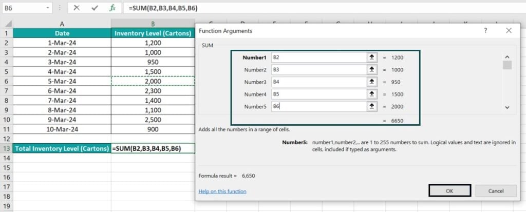

Once all argument values are updated, click OK to achieve the required sum value.]
The SUM() accepts the per-day inventory level figures in the cells B2:B11 in rows 2 to 11 as the input. It then adds the values to return 14,850 as the required total inventory level.
Example #2 – Sum Multiple Rows To Single Cell
The source dataset contains the monthly revenue data at four branch offices of a firm in rows 2 to 7 of columns B to E.

The task is to evaluate the total revenue and display the output in cell B9, where the data format is set as Currency in the Number Format option in the Home tab.
In this case, we must sum multiple rows and columns in Excel to fetch the required total revenue figure, which we can do using the SUM() as explained below:
Step 1: Choose cell B9, enter the SUM(), and press Enter.
=SUM(B2:E7)

The SUM() adds all the numeric values in the specified range, which spans across multiple rows and columns, to return the required total revenue value of $512,000.
Example #3 – Select Entire Row As The Reference
The source dataset includes the copies sold data of two books from 2015-23.

The requirement is to compute the total copies of the two books sold based on the input data and show the output in cell B7.
Then, we can use the SUM() in the target cell to secure the required output by supplying the entire row reference as the input to the function.
Step 1: Select cell B7 and enter the SUM().
=SUM(A3:A4

Next, press Shift + Space Bar to get the reference to the two entire rows.
=SUM(3:4

Next, close the bracket.

Step 2: Press Enter to view the SUM() return value.

Initially, we select the column A cells in rows 3 and 4 as the input in the SUM(). We do so as the required data we intend to add is in rows 3 and 4, and the shortcut enables us to select the two whole rows quickly.
Finally, the function adds all the numbers in the two chosen rows to return 94,500 as the required count of total copies sold.
Important Things To Note
- Ensure to enter the SUM() name correctly to sum multiple rows in Excel. Otherwise, the function return value will be the #NAME error value.
- Ensure the numbers supplied as input to the SUM() are not formatted as Text. Otherwise, the function will ignore such values while adding the data points, leading to it returning an incorrect value.
- Ensure the SUM() formula does not contain any Excel circular reference. Otherwise, the function output will be 0.

Frequently Asked Questions (FAQs)
We can SUMIF to sum multiple rows using the following steps, explained with an example.
The source dataset contains the zonal sales figures for different products at a firm.
The task is to calculate the total sales generated in the North zone and display the output in cell D13. Also, the target cell has its data format set as Currency in the Number Format option in the Home tab.
Then, here is how we can use the SUMIF() in the target cell to achieve the required sum value based on the cited condition.
Step 1: Select cell D13, enter the SUMIF(), and press Enter.
=SUMIF(A2:A11,”North”,D2:D11)
First, the function checks for cells in the range A2:A11 that contain the phrase North, which are cells A2, A4, and A10. Next, the function adds the sales figures in the corresponding rows of column D, in the range D2:D11, which are the cells D2, D4, and D10 values. Thus, we get the value of $38,000 as the required total sales figure for the North zone.
The shortcut to sum multiple rows in Excel is Alt + =, and the steps to use the shortcut are as follows:
1. Place the mouse cursor after the column of values we aim to add (or on the left of the row of values we aim to sum).
2. Press the Alt key. After that, press the ‘=’ sign while still pressing Alt.
3. Press Enter to complete the action.
You can sum multiple rows in Excel that are not next to each other using the following steps:
1. Choose the cell where you want to display the total.
2. Type =SUM( into the cell.
3. Select the first cell containing the required data you want to add.
4. Hold the Ctrl key while clicking the remaining cells in the other concerned rows. 5. The formula will show all the selected cell references, separated by commas.
6. Close the bracket to complete the expression and press Enter to view the sum of values in multiple rows that are not next to each other.
Download Template
📥Download the ready-to-use Excel template to practice this tutorial yourself.
How-to-Sum-Multiple-Rows-in-Excel-TemplateRecommended Articles
Guide to How To Sum Multiple Rows In Excel? Here we learn top 3 methods to sum multiple Excel rows with examples and points to remember. You can learn more from the following articles –

Leave a Reply