Interpolate In Excel

What Is Interpolate In Excel?

Interpolate in Excel or Interpolation helps users to evaluate or forecast an unknown value that lies between two known data points in a dataset. The graphical representation is related to the data points such as noise level, rainfall, elevation, etc.

The Interpolate Excel is an inbuilt Statistical function with the name as Forecast, so we can insert the formula from the “Function Library” or enter it directly in the worksheet.

For example, the image below depicts the values, and we will calculate using the Interpolate formula, i.e., the Forecast formula.

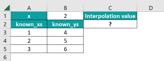
Select cell C2, enter the formula =FORECAST(B1,B3:B5,A3:A5), and press “Enter”.

The result is ‘5’, as shown above using the Linear graph.

What Is Interpolate In Excel?

Interpolate in Excel is the process used to predict or derive values between the given values.
We can calculate the Interpolation for a dataset using the Forecast function with the same size cell ranges for the x and y values.
The different types of Interpolates are Piecewise Constant Interpolation, Linear Interpolation, Polynomial Interpolation, Spline Interpolation, and Mimetic Interpolation.
Linear Interpolation is used to predict values for rainfall, geographical data points, etc.
We can calculate the Interpolate mathematically using the formula, y = y1 + (x – x1) ⨯ (y2 – y1) / (x2 – x1).

Interpolate Excel Formula

Linear Interpolation – This method is quick and easy to use, also known as Lerp. To perform the Linear Interpolate calculations, we use the FORECAST Excel formula.

The syntax of the FORECAST Excel formula is,

Interpolate in Excel - FORECAST Excel Formula

The three mandatory arguments of the FORECAST Excel formula are,

x: It is the predicted value.
known_ys: It is a dependent value in the dataset.
known_xs: It is an independent value in the dataset.

Excel VBA – All in One Courses Bundle (35+ Hours of Video Tutorials)

If you want to learn Excel and VBA professionally, then Excel VBA All in One Courses Bundle (35+ hours) is the perfect solution. Whether you’re a beginner or an experienced user, this bundle covers it all – from Basic Excel to Advanced Excel, Macros, Power Query, and VBA.

Start Learning Now

How To Interpolate in Excel?

We can find Interpolate in Excel using 2 ways, namely,

Access from the Excel ribbon.
Enter in the worksheet manually.

Method #1 – Access from the Excel ribbon

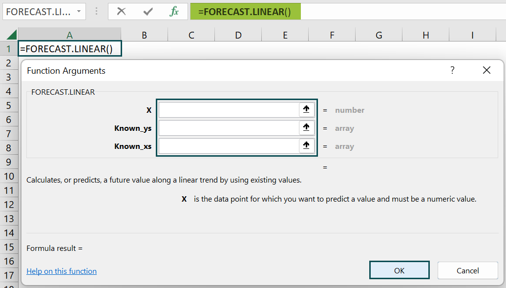
Choose an empty cell → select the “Formulas” tab → go to the “Function Library” group → click the “More Functions…” option drop-down → select the “Statistical” option right arrow → select the “FORECAST.LINEAR” option, as shown below.

Interpolate in Excel - Access from the Excel ribbon

The “Function Arguments” window appears. Enter the arguments in the “X”, “Known_ys”, and “Known_xs” fields, and click “OK”.

Interpolate in Excel - Function arguments window

Method #2 – Enter in the worksheet manually

Select an empty cell for the output.
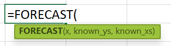
Type =FORECAST( in the selected cell. [Alternatively, type =F or =FORE and double-click the FORECAST.LINEAR Interpolate function from the list of suggestions shown by Excel.
Enter the arguments as cell values or cell references and close the brackets.
Press the “Enter” key.

Let us take a basic example to learn this function.

We will calculate the interpolation using the FORECAST function for the value of x & y.

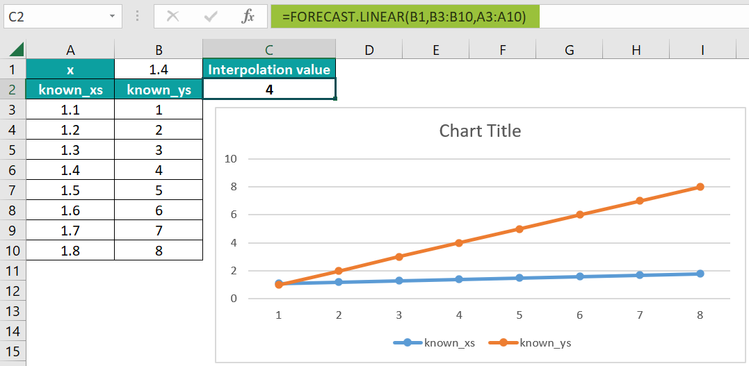
In the table, the data is,

Cell B1 contains the x values.
Column A contains the known_xs values.
Column B contains the known_ys values.

How to Use Interpolate in Excel - Basic Example

The steps to calculate the Interpolation in excel using the FORECAST formula are,

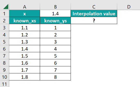
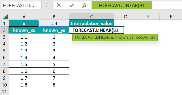
Select cell C2, and enter the formula =FORECAST.LINEAR(B1, i.e., x argument value.
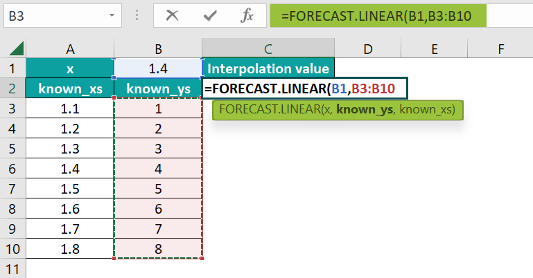
The entered value of the known_ys argument in cells “B3:B10”. The formula now is =FORECAST.LINEAR(B1,B3:B10
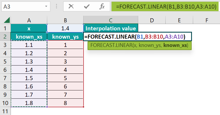
Enter the value of the known_xs argument as “A3:A10”, and close the brackets. The complete formula is =FORECAST.LINEAR(B1,B3:B10,A3:A10).
Press the “Enter” key. The calculated result is “4”, as shown below, along with a graph.

Examples

We will consider some advanced scenarios for Interpolate in Excel using the Forecast formula.

Example #1

We will calculate the Interpolate using the FORECAST function for the value of time and distance in columns.

In the table, the data is,

Cell B1 contains the x values.
Column A contains the known_xs values.
Column B contains the known_ys values.

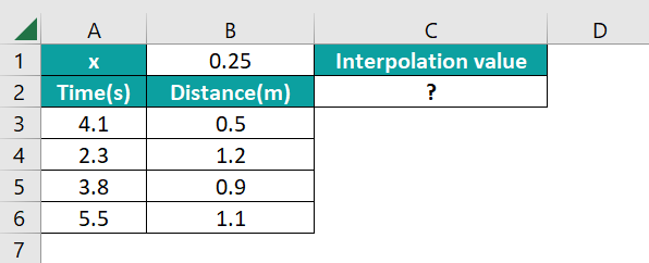
The procedure to calculate the Interpolate in Excel using the FORECAST formula is,

Select cell C2, enter the formula =FORECAST.LINEAR(B1,B3:B6,A3:A6), and press “Enter”.

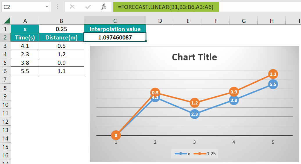
The calculated result is “1.097460087”, as shown above along with the graph.

Example #2

We will calculate the Interpolate using the FORECAST function for thevalue of monthly sales & quantity of ABC company.

In the table, the data is,

Cell B1 contains the x values.
Column A contains the known_xs values.
Column B contains the known_ys values.

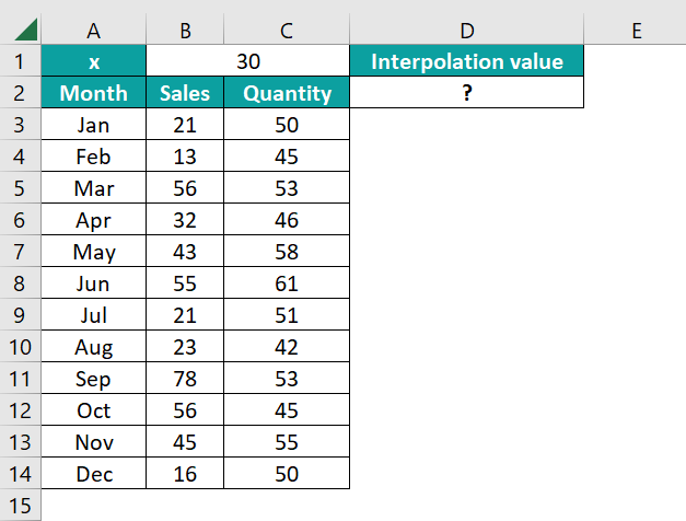
The procedure to calculate the Interpolate in Excel using the FORECAST formula is,

Select cell D2, enter the formula =FORECAST.LINEAR(B1,C3:C14,B3:B14), and press “Enter”.

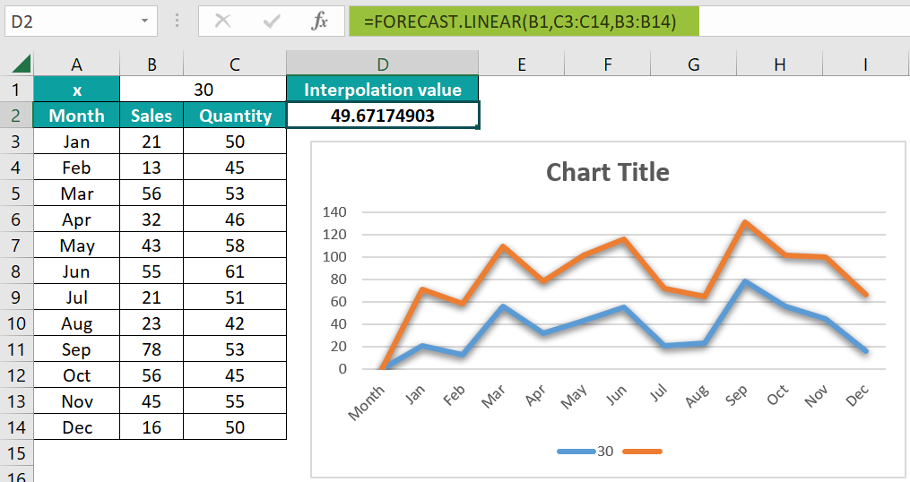
The calculated result is “49.67174903”, as shown above along with the graph.

Example #3

We will calculate the Interpolate using the FORECAST function for thevalue of x and y.

In the table, the data is,

Cell B1 contains the x values.
Column A contains the known_xs values.
Column B contains the known_ys values.

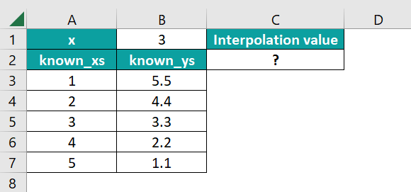
The procedure to calculate the Interpolate using the FORECAST formula is,

Select cell C2, enter the formula =FORECAST.LINEAR(B1,B3:B7,A3:A7), and press “Enter”.

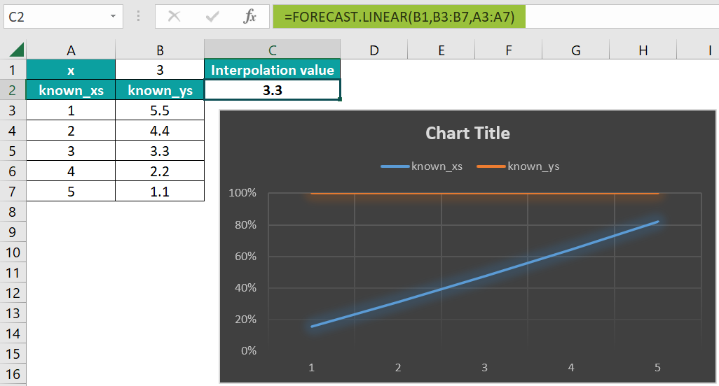
The calculated result is “3.3”, as shown above along with the graph.

Important Things To Note

Interpolation using the Forecast is commonly used because it is fast and precise, easy to use, and time-saving if the table values are closely spaced.
This method is used to evaluate values for geographical data points.
If the cell ranges of the known_xs and the known_ys argument values are not the same sizes, we will get the “#NA” error.

Frequently Asked Questions (FAQs)

1. What does the Linear Interpolate function do in Excel?

Linear Interpolation helps users understand the relationship between x and y coordinates on datasets and graphs, and uses them to estimate new coordinates. The FORECAST function is used to calculate Linear Interpolate in Excel.

2. How does the Interpolate function work in Excel?

We can work with the Interpolate function as follows:

1) Select an empty cell for the output.
2) Type =FORECAST( in the selected cell. [Alternatively, type =F or =FORE and double-click the FORECAST.LINEAR Interpolate function from the list of suggestions shown by Excel.
3) Enter the arguments as cell values or cell references and close the brackets.
4) Press the “Enter” key.

For instance, we will calculate the Interpolate in Excel using the FORECAST function for thevalue of x and y.

In the table, the data is,
• Cell B1 contains the x values.
• Column A contains the known_xs values.
• Column B contains the known_ys values.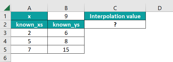

The procedure to calculate the Interpolate in Excel using the FORECAST formula is,

Select cell C2, enter the formula =FORECAST.LINEAR(B1,B3:B5,A3:A5), and press “Enter”.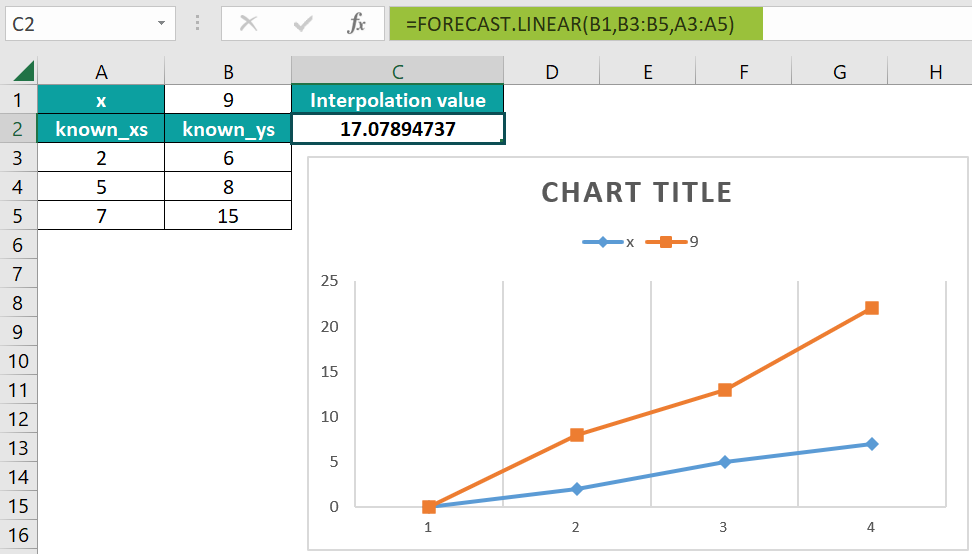

The calculated result is “17.07894737”, as shown above with the graph.

3. Where is the Interpolate Function in Excel?

The Interpolate in Excel’s Forecast formula is found as shown below.
Choose an empty cell → select the “Formulas” tab → go to the “Function Library” group → click the “More Functions…” option drop-down → select the “Statistical” option right arrow → select the “FORECAST.LINEAR” option, as shown below.

Download Template

This article must help understand the Interpolate In Excel formula and examples. You can download the template here to use it instantly.

Interpolate In Excel Download

Interpolate In Excel