
What Is ISERROR In Google Sheets?
ISERROR function in Google sheets, as the name suggests, helps users find if a value in a cell is an error or not. It is a default function and it is available in both Excel and Google sheets. Remember, the ISERROR function returns TRUE if the value in the active cell is an error. Similarly, if the value is not an error, the ISERROR function returns FALSE.
For example, consider the below table showing value and result in columns A and B, respectively.

Now, let us learn how to use the ISERROR function to find the result in column B. To begin with, select the cell B2 and enter the ISERROR function formula, =ISERROR(A2) and press Enter key.
We will be able to see the result in cell B2. Likewise, using Autofill option, we will be able to see the result in cell B3, as shown in the below image.

In this article, let us learn how to use ISERROR function with detailed examples.
Use this ISERROR In Google Sheets Template to follow along with the examples in this article.
Download Excel TemplateKey Takeaways
- ISERROR function in Google sheets is a function used to find the cells containing the error in the given data or a specific cell.
- The syntax of ISERROR function in Google sheets is =ISERROR(value) where value is the mandatory argument showing the cell for which we want to test whether it is an error or not.
- The function is an default function available in both Excel and Google sheets.
- Remember, using this function, we can validate user input, check for errors in the formula and filter out errors from data sets.
ISERROR() Google Sheets Formula

The formula of ISERROR Google sheets function is =ISERROR(value)
where
- value is the only mandatory argument which refers to the cell for which we want to test if it’s an error or not.
How To Use ISERROR Function In Google Sheets?
We can use the ISERROR function in two ways. They are:
- Select the ISERROR function under the Insert tab
- Manually enter the ISERROR function
Method #1 – Select the ISERROR function under the Insert tab
The steps to select the ISERROR function in Google sheets under the Insert tab are:
Step 1: To begin with, we need to insert the data in Google sheets. Next, select the cell where we want to enter the formula.
Step 2: Next, select the Insert tab and then, click on the Function option. Then, click on the Info option drop-down.
Step 3: Now, click on the ISERROR function.

Step 4: We will be able to see the formula in the active cell. Next, we need to select the cells as argument for the function.
Step 5: Press Enter key. We will be able to see the result in the active cell.
Likewise, we can use the ISERROR function in Google sheets using the Insert tab.
Method #2 – Manually enter the ISERROR function in Google Sheets
The steps to manually enter the ISERROR function are:
Step 1: To begin with, we need to insert the data in Google sheets. Next, select the cell where we want to enter the formula.
Step 2: Next, type ISERROR function. Proceed to the next step.
Step 3: Alternatively, we can also type =ISER and select the ISERROR function in Google sheets.

Step 4: We will be able to see the formula in the active cell. Next, we need to select the cells as argument for the function.
Step 5: Press Enter key. We will be able to see the result in the active cell.
Likewise, we can use the ISERROR function in Google sheets by manually entering the function.
Examples
Now, let us learn how to use the ISERROR function.
Example #1 – Basic Example
For example, consider the below table showing value and result in columns A and B, respectively.

Now, let us learn how to use the ISERROR function in Google sheets to find the result in column B.
The steps are:
Step 1: To begin with, we need to enter the data in the cell range. In this example, the data is available in the cell range A1:B5. Next, we need to select the cell where we want to find the result. In this example, we need to select the cell B2.
Step 2: Next, enter the ISERROR function formula.
So, the complete formula is =ISERROR(A2).
Step 3: Press Enter key.
We will be able to see the result in cell B2, as shown in the below image.

Step 4: Next, using Autofill option, we will be able to see the result in the cell range B3:B5, as shown in the below image.

Likewise, we can use ISERROR function to find the values containing errors in the data.
Example #2 – Using ISERROR To Return New Value Instead Of An Error Code
For example, consider the below table showing values 1 and 2 in columns A and B, respectively.

Now, let us learn how to use the ISERROR function to find the result in column C.
The steps are:
Step 1: To begin with, we need to enter the data in the cell range. In this example, the data is available in the cell range A1:C5. Next, we need to select the cell where we want to find the result. In this example, we need to select the cell C2.
Step 2: Now, we need to use ISERROR to return new value instead of an error code. For this, we need to use IF function along with ISERROR function.
So, the complete formula is =IF(ISERROR(A2/B2), “Incorrect”, A2/B2).
Step 3: Press Enter key.
We will be able to see the result in cell C2, as shown in the below image.

Step 4: Next, using Autofill option, we will be able to see the result in the cell range C3:C5, as shown in the below image.

Likewise, we can use ISERROR function in Google sheets to find the values containing errors in the data such that we can return new value instead of an error code.
Example #3 – Using ISERROR With VLOOKUP
For example, consider the below table showing name and region in columns A and B, respectively.

Now, let us learn how to use the ISERROR function in Google sheets with VLOOKUP to find the result in column D.
The steps are:
Step 1: To begin with, we need to enter the data in the cell range. In this example, the data is available in the cell range A1:B5. Next, we need to select the cell where we want to find the result. In this example, we need to select the cell D2.
Step 2: Assume that we have to find the person named ‘Rob’ in the data. For that, we need to enter the ISERROR function formula along with VLOOKUP and IF functions.
So, the complete formula is =IF(ISERROR(VLOOKUP(“Rob”, A1:B5, 2, FALSE)),”Not available”, VLOOKUP(“Rob”, A1:B5, 2, FALSE)).
Step 3: Press Enter key.
We will be able to see the result in cell D2, as shown in the below image.

Likewise, we can use ISERROR function in Google sheets along with VLOOKUP and IF functions to find the data.
Example #4 – Using The ISERROR Function In An Array Formula To Handle Errors
For example, consider the below table showing product, price, profit and result in columns A, B, C and D, respectively.

Now, let us learn how to use the ISERROR function to find the result in column D with array formula.
The steps are:
Step 1: To begin with, we need to enter the data in the cell range. In this example, the data is available in the cell range A1:C5. Next, we need to select the cell where we want to find the result. In this example, we need to select the cell D2.
Step 2: Next, enter the ISERROR function formula.
So, the complete formula is =ArrayFormula(IF(ISERROR(C2:C5/B2:B5),”ERROR VALUE”,C2:C5/B2:B5)).

Step 3: Press Enter key.
We will be able to see the result in cell D2, as shown in the below image.

Likewise, we can use ISERROR function in Google sheets with array formula.
Important Things To Note
- ISERROR is an inbuilt Google sheets function used to find whether the cell containing the value is an error or not.
- We can use this function to find which cell is having the error. This is highly useful, especially when working with huge datasets.
- Some of the functions similar to ISERROR function in Google sheets are IFERROR, ISNA and ISTEXT functions in Google sheets.
Frequently Asked Questions (FAQs)
For example, consider the below table showing value and result in columns A and B, respectively.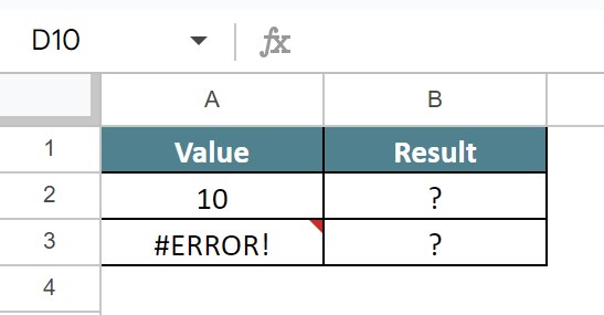
Now, let us learn how to use the ISERROR function in Google sheets to find the result in column B.
The steps are:
Step 1: To begin with, we need to enter the data in the cell range. In this example, the data is available in the cell range A1:B5. Next, we need to select the cell where we want to find the result. In this example, we need to select the cell B2.
Step 2: Next, enter the ISERROR function formula in Google sheets.
So, the complete formula is =ISERROR(A2).
Step 3: Then, press Enter key.
Now, we will be able to see the result in cell B2, as shown in the below image.
Step 4: Next, using Autofill option, we will be able to see the result in the cell B3, as shown in the below image.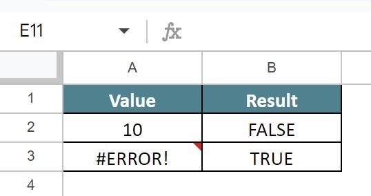
Likewise, we can use ISERROR function to find the values containing errors in the data.
The difference between ISERR and ISERROR functions in Google sheets are:
• ISERR function in Google sheets helps users find whether a value is an error, other than #N/A error.
• On the other hand, ISERROR Google sheets function, finds whether the value in the cell is an error or not. This function includes #N/A error also.
The ISERROR function in Google sheets may not work properly if the value in the formula does not match with the arguments entered in the formula. Similarly, the function does not work if there is a missing value or any incorrect function name.
Use this ISERROR In Google Sheets Template to follow along with the examples in this article.
Download Excel Template