
What Is MODE.MULT Excel Function?
The MODE.MULT Excel function is a statistical tool used to find the most frequently occurring values in data with multiple modes. The MODE function is used to detect the first mode, but the MODE.MULT gives an array of all modes presented in the data.
The MODE.MULT function mainly works with datasets that exhibit more than one leading value. Using this function, we can study our data deeply and make conversant opinions based on correct, consistent study. If there is only one mode in a data set, we get a single result from MODE.MULT Excel, which is the value making the maximum appearances.
Use this MODE.MULT Excel Template to follow along with the examples in this article.
Download Excel TemplateIn the following example, we will explore the values entered and determine the mode from the dataset using the MODE.MULT Excel function.

To begin, enter the formula with the set of numbers directly in cell B2. Once the formula is entered, press the CTRL + SHIFT + Enter keys to obtain the desired outcome.
{=MODE.MULT(1,1,1,1,2,2,2,2,3,3,3,4,4,5)}
Instead of using just the Enter key, we use this combo of keys when working on complex calculations in array formulas, as in the above case. Your formula will be enclosed in {} to indicate it is an array formula. The result will be an array of values in such cases.
The results will be displayed in cells B2 and B3, visually represented as 1 and 2, respectively.

CTRL + SHIFT + Enter is used in the conversion of data into an array format comprising multiple data values. This feature also enables the distinction between regular formulas and array formulas in Excel. Array excel formulas can be categorized into two types: those that have a single result and those that have multiple results.
Syntax
The MODE.MULT Excel function utilizes the following arguments:
- number1 – This is a required argument. It is the cell reference of the array or numeric values.
- number2 – This is an optional argument, which again is a number or cell reference referring to numeric values.
How To use MODE.MULT Function in Excel?
To effectively utilize the MODE.MULT Excel function, follow these steps.
#1 – Access from the Excel ribbon
Step 1: Choose an empty cell to type the formula. Go to the “Formulas” tab and click on it.

Step 2: Select the “More Functions” option from the menu.

Step 3: Select the “Statistical” option from the drop-down list. Select “MODE.MULT” from the drop-down menu.

Step 4: A window called “Function Arguments” appears. Enter the values for the “number1” and “number2” arguments, respectively.
Select OK.

#2 – Enter the worksheet manually.
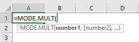
Step 1: Select an empty cell to type the MODE.MULT Excel function. Type “=MODE.MULT (” in the selected cell, enter the arguments, and close the braces. Alternatively, type “=M” and double-click the MODE.MULT Excel function from the list of suggestions shown by Excel.

Step 2: Press the “Enter” key to get the result.

Examples
Example #1 – Passing Direct Numerical Values as the Function argument
Let us use the example to understand the functionality of the MODE.MULT function in Excel.
We will be passing Direct Numerical Values as the Function argument. Consider the data 1,1,2,2,2,3,3,3,4,4,5,5,5. To apply the MODE.MULT Excel function, please follow these steps:

Step 1: Begin by selecting cell B3 to enter the formula.
Step 2: Enter the formula with the frequency of values.
=MODE.MULT(1,1,2,2,2,3,3,3,4,4,5,5,5)

Step 3: As a result, we will obtain the value of 2, as shown below. We have selected only one cell for the output, so the function returns the first mode number; we will select more cells and enter the formula. The function will return the output in ascending order.

Example #2 – Using MODE.MULT with multiple ranges.
Let us use the following example to understand the MODE.MULT function in Excel. In this case, we will be using MODE.MULT with multiple ranges to find the most repeated values in the two datasets. Given below is a table containing different sets of data in columns A and B.

To effectively apply the MODE.MULT function in Excel, please adhere to the following steps:
Step 1: Select the cell E4, where we will input the formula. Enter the formula that represents the frequency of values and enter two sets of arguments.
=MODE.MULT(A2:A9, B2:B9)

Step 2: Press CTRL + SHIFT + Enter keys and attain the result in cells E4 & E5 as 10 & 5, as visually depicted below.
These are the most occurring values in the two data sets, A2 to A9 and B2 to B9.

Example #3 – Passing Cell Ranges as Numerical Data Set
To understand the MODE.MULT Excel function, let us investigate the following example where we have specific serial numbers assigned to different subjects in a school.
Students take a quiz on any subject of their choice and fill in the serial number and subject name. We can find the most popular quiz taken by the students using the MODE.MULT Excel function.

To effectively implement the MODE.MULT function in Excel, it is crucial to follow these steps:
Step 1: Begin by selecting cell F8, where we will input the formula.
Step 2: Proceed to enter the formula that represents the frequency of values.
= (MODE.MULT(C2:C15)

Step 3: To obtain the desired outcome, press the Enter key. The result will be generated in cell F8. We observe that the subject in which most students attempted the quiz was English.

It is because we get a result of 1 in F8, which indicates the most repeated number and is the serial number of English.
Example #4
Now, let us look at an example of what happens if the data contains values in different formats. To implement the MODE.MULT function in Excel successfully, it is crucial to follow below steps:

Step 1: Begin by selecting cells B2 and E2, where we will input the formula.
Step 2: Proceed to enter the formula that represents the frequency of values.
In cell B2, enter the formula =MODE.MULT(1,1,7,A,7,7,4,3)
It is a direct formula, and using this, the function will check each value.
In cell E2, enter the formula =MODE.MULT(D2:D9)
It contains an array range, which will omit the string value.
Step 3: To obtain the desired outcome, press the Enter key. The result will be generated in cells B2 and E2, visually depicted in the below image.

- Therefore, in first case, the #NAME! Error occurs because a non-numeric value is entered as input to the function.
- In the second case, the MODE.MULT function ignores non-numeric functions that are part of an array of values.
Important Things To Note
- The #N/A! error occurs when there are no repeated values of the entered values.
- The #VALUE! error occurs when a non-numeric value is entered as input to the function. The MODE.MULT function ignores non-numeric functions that are part of an array of values.
- The errors will occur if the value entered is the error value or any text value that cannot be modified into a numeric value.
- The MODE.MULTfunction can only have numbers or names, arrays, or reference cells that contain numeric values as entered values.
- If the value in the array is text, logical values, or empty cells, then the values will be overlooked.
- The Excel MODE.MULT function was introduced in Excel 2010 and is not accessible in earlier versions of the software.
Frequently Asked Questions (FAQs)
The MODE.MULT function used for calculating frequently occurring values. The function lets users determine the multiple modes in the dataset. This function can handle large amounts of data and mixed data types. It is mainly used in dealing with complex datasets that have more value. It shows a comprehensive view of the variations and patterns in the datasets. In the following example, you have different types of values. You can find the mode from the data set using MODE.MULT Excel function.
Enter the formula that represents the frequency of values in two cells, E3 & E4 and press the Enter key.
=MODE.MULT(A2:A9)
=MODE.MULT(B2:B9)
The results in cells E3 and E4 are visually depicted as 10% and 1, respectively.
The major difference between the MODE and MODE.MULT functions in Excel are to handle multiple modes or frequencies of occurring values in the datasets.
The MODE function returns the single most frequently occurring values, whereas the MODE.MULT function returns multiple modes occurring most frequently of an array of all values.
The MODE.MULT function is used when there is more than one mode, while the MODE function returns only one mode.
The MODE.SNGL and MODE.MULT functions in Excel are both used to calculate the mode of a dataset, with the different ability to solve multiple modes.
The MODE.MULT function finds multiple modes by returning an array of all values that occur most frequently. This makes it particularly useful when dealing with data sets containing several repeated values.
The MODE.SNGL function finds a single mode, which represents the value that occurs most frequently in a given set of data. In case there is more than one value that occurs most frequently, this function will return an error.
One can activate the Excel MODE.MULT Function by choosing the “MODE.MULT” function by going to the “Formulas” tab -> “More Functions” option -> “Statistical” option
A window called “Function Arguments” appears and enter the arguments. Select OK.
Use this MODE.MULT Excel Template to follow along with the examples in this article.
Download Excel Template